Overview
Teaching: 0 min
Exercises: 0 minQuestions
Key question
Objectives
First objective.
Quality assessment / quality control of a single dataset
Recap so far
Our computing environment
We’re using the dataCgen-qc (ami-3c1c3454) Amazon Machine Image for this analysis. The directory structure looks like this:
/home/ec2-user/
└── data
    ├── FastQC
    │   ├── fastqc                *** the fastqc executable
    │   └── ...                   *** other FastQC files and folders omitted for clarity***
    ├── SRR                       *** This is the folder that contains our data
    │   ├── SRR447649_1.fastq
    │   ├── SRR447649_2.fastq
    │   ├── SRR447649_3.fastq
    │   ├── SRR519926_1.fastq     *** These are the read files we will use.
    │   └── SRR519926_2.fastq     *** These are the read files we will use.
    └── Trimmomatic-0.32
        ├── adapters
        ├── LICENSE
        └── trimmomatic-0.32.jar  *** The trimmomatic java program
To learn how to log in, please review the previous lesson on logging in to a cloud instance. Specifically, you’ll need to obtain the public DNS of your personal cloud instance, and a “key” file. You’ll need to modify the permissions of your key file and log in to your cloud instance (instructions for mac and Windows, but note, username should be ec2-user, not ubuntu or root, as these instructions say).
Our data
First, let’s take a look around. Go into the data/SRR folder, and list the contents.
pwd
cd ~/data/SRR
The run that starts with SRR519926 is a paired-end 2x250bp MiSeq run on Escherichia coli str. K-12 substr. MG1655. You can learn more about it by searching for SRR519926 in the Sequence Read Archive. If you click on the name of the run, you’ll see details such as the number of reads (~400,000), total number of base pairs, file size, GC content, etc.
Since this was done several years ago when 2x250 reads were relatively new, I would expect the quality to degrade rather severely toward the end of the reads. There may also be some other issues that we’re unaware of. Let’s take a look at the quality of the data with FastQC.
Quality assessment
Check available resources
- Use
topto determine whether other resources are being run at the moment - Do you have enough resources for your work?
top - 14:42:44 up  1:28,  1 user,  load average: 0.00, 0.01, 0.05
Tasks:  68 total,   1 running,  67 sleeping,   0 stopped,   0 zombie
Cpu(s):  0.2%us,  0.0%sy,  0.0%ni, 99.8%id,  0.0%wa,  0.0%hi,  0.0%si,  0.0%st
Mem:   4050732k total,  2587536k used,  1463196k free,    49464k buffers
This tells us that the CPU usage is 0.2% (third line) and we have about 4GB of RAM on the machine with ~1.5GB free. This should be enough to run a quality assessment with FastQC.
Run FastQC
Currently, the default-installed FastQC program doesn’t function properly, so we downloaded and extracted a new version in the ~/data/FastQC directory in your home.
# Run fastqc and get some help and version information
~/data/FastQC/fastqc -h
~/data/FastQC/fastqc -v

# Now run it on your samples
mkdir qc
~/data/FastQC/fastqc SRR519926_*.fastq --outdir qc
(Note: If they are taught (and they probably should be) the output dir should follow the same data organization standards talked about (or that will be discussed) in the data organization module).
Transferring FastQC Results
Note that the output is in a specific output directory, and is present at both an HTML file and a *.zip file.
cd qc
ls -l
The results are presented in an HTML file, but we can only open HTML files in browser, so we need to transfer this data back to our local machine and open it in chrome or firefox or something.
One way to do this is using the command line:
# On your remote server, where is your data?
pwd

# On your laptop:
scp -i /path/to/key.pem username@ipaddress:~/path/to/html/file.html /some/local/directory
# e.g., copy to here (".")
scp -i ~/key.pem ec2-user@123.45.67.890:/home/ec2-user/data/SRR/qc .
Alternatively, we could use a file transfer client (e.g., https://cyberduck.io/) to transfer the data graphically, as in the instructions here. Essentially, you’ll want to open a new SFTP connection to the DNS address you were given using the key file to “get into” the instance and transfer the data.
Interpreting FastQC results
Let’s have a look at the results. This is the boxplot analysis for your FASTQ data. Phred quality score is on the ordinate axis. The purpose of this plot is to look at the overall quality of the sequence.
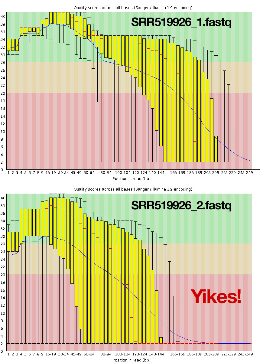
This indicates very poor quality toward the end of the reads. You can also look at lots of other quality issues, including potential adapter contamination, and over-represented kmers near the beginning of the read. Contrast this to a good sequencing run.
Preview: What if you had 20 files to QC? 200? 2,000? See the next lesson on parallel analyses.
Trimming and filtering your sequence data
We’re going to use a tool called Trimmomatic to trim and filter our sequence data.
- Paper: Bolger, Anthony M., Marc Lohse, and Bjoern Usadel. “Trimmomatic: a flexible trimmer for Illumina sequence data.” Bioinformatics (2014) 30(15):2114-20 doi:10.1093/bioinformatics/btu170. (On PubMed Central).
- Software: http://www.usadellab.org/cms/?page=trimmomatic
- Manual: http://www.usadellab.org/cms/uploads/supplementary/Trimmomatic/TrimmomaticManual_V0.32.pdf
Trimmomatic is a fast, multithreaded command line tool that can be used to trim and crop Illumina (FASTQ) data as well as to remove adapters.
The FastQC report above found evidence of adapter contamination, but adapter removal is a bit tricky so we’re going to skip that here (but you should check out the manual above and try it on your own using the TruSeq-3-PE-2.fa adapter file in the Trimmomatic directory).
First, let’s create a new directory where we will store our trimmed reads.
mkdir SRR519926_trimmed
cd SRR519926_trimmed
Now, let’s run trimmomatic without any arguments and get some help (run it with java, giving it the full path to the trimmomatic jar file):
java -jar ~/data/Trimmomatic-0.32/trimmomatic-0.32.jar
This gives us some help:
Usage:
       PE [-threads <threads>] [-phred33|-phred64] [-trimlog <trimLogFile>] [-basein <inputBase> | <inputFile1> <inputFile2>] [-baseout <outputBase> | <outputFile1P> <outputFile1U> <outputFile2P> <outputFile2U>] <trimmer1>...
   or:
       SE [-threads <threads>] [-phred33|-phred64] [-trimlog <trimLogFile>] <inputFile> <outputFile> <trimmer1>...
Since we have paired end data, we must use PE mode. We’ll specify that we’re using phred33 quality scores. For paired-end data, two input files, and 4 output files are specified, 2 for the ‘paired’ output where both reads survived the processing, and 2 for corresponding ‘unpaired’ output where a read survived, but the partner read did not. Finally, we give trimmomatic some trimmer keywords. We’ll talk about those below:
java -jar ~/data/Trimmomatic-0.32/trimmomatic-0.32.jar PE \
  -phred33 -trimlog trimlog.txt \
  ../SRR519926_1.fastq ../SRR519926_2.fastq \
  p1.fq u1.fq p2.fq u2.fq \
  LEADING:5 TRAILING:5 SLIDINGWINDOW:4:20 MINLEN:50
java -jar ~/data/Trimmomatic-0.32/trimmomatic-0.32.jar: Run trimmomaticPE: in paired end mode-phred33: Using Phred33/Sanger/Illumina 1.9 quality score encoding.-trimlog trimlog.txt: Logging to a file called trimlog.txt a list of all read trimmings, including the read name, surviving length, location of the first and last surviving bases, and the amount trimmed from the end of the read.../SRR519926_1.fastq ../SRR519926_2.fastq: using these fastq input filesp1.fq u1.fq p2.fq u2.fq: saving paired surviving reads in p1.fq and p2.fq, and unpaired reads in u1.fq and u2.fqLEADING:5: Removing low-quality bases from the beginning if they pass below this thresholdTRAILING:5: Removing low-quality bases from the end if they pass below this thresholdSLIDINGWINDOW:4:20: Perform a sliding window trimming, cutting once the average quality within the a 4-bp window falls below quality score of 20. By considering multiple bases, a single poor quality base will not cause the removal of high quality data later in the read.MINLEN:50: Trash reads completely if their surviving length is less than 50bp.
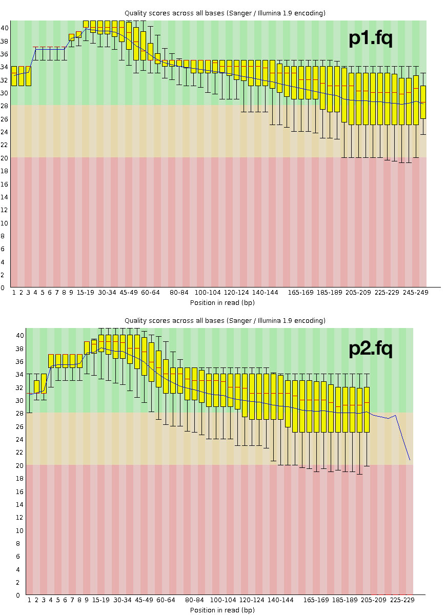
Exercise: Re-run FastQC on the new paired surviving reads, p1.fq and p2.fq. Transfer them and open them up for viewing.
The trimmed data look much better, but you might still want to consider going back and trimming adapters.
Key Points
First key point.