Learning Objectives
Following this assignment students should be able to:
- install and load an R package
- understand the data manipulation functions of
dplyr- execute a simple import and analyze data scenario
Reading
Readings
Optional Resources:
- Data Analysis and Visualization in R for Ecologists - Working with data
- dplyr vignette
- Mapping between dplyr and base R
Lecture Notes
Setup
install.packages(c('dplyr', 'readr', 'tidyr'))
download.file("https://ndownloader.figshare.com/files/2292172",
              "surveys.csv")
download.file("https://ndownloader.figshare.com/files/3299474",
              "plots.csv")
download.file("https://ndownloader.figshare.com/files/3299483",
              "species.csv")
download.file("https://www.datacarpentry.org/semester-biology/data/shrub-volume-data.csv",
              "shrub-volume-data.csv")
download.file("https://www.datacarpentry.org/semester-biology/data/shrub-volume-experiments.csv",
              "shrub-volume-experiments.csv")
download.file("https://www.datacarpentry.org/semester-biology/data/shrub-volume-sites.csv",
              "shrub-volume-sites.csv")
download.file("https://datacarpentry.org/semester-biology/data/mbaiki_measures.csv",
              "mbaiki_measures.csv")
download.file("https://datacarpentry.org/semester-biology/data/mbaiki_trees.csv",
              "mbaiki_trees.csv")
download.file("https://datacarpentry.org/semester-biology/data/mbaiki_species.csv",
              "mbaiki_species.csv")
download.file("https://datacarpentry.org/semester-biology/data/penguins_no_na.csv",
              "penguins_no_na.csv")
Lecture Notes
- dplyr Aggregation
- dplyr Joins
- Converting between data frames and vectors
- AI - Introduction and Basic Prompting
Exercises
Penguins Data Aggregation (5 pts)
If the file
penguins.csvis not already in your working directory then download it into your working directory.Load
penguins.csvinto R usingread_csv().- Use the
group_by()andsummarize()functions to get a count of the number of individuals in each species. - Use the
drop_na(),group_by(), andsummarize()functions to calculate the averagebill_length_mmfor each species. - Use the
drop_na(),group_by(), andsummarize()functions to calculate the maximumflipper_length_mmfor each species on each island. - Use the
filter(),drop_na(),group_by(), andsummarize()functions to get the mean body mass of Chinstrap penguins on each island. - Find the mean bill ratio (bill length / bill depth) for each species on each island.
- Use the
Portal Data Aggregation (5 pts)
If the file surveys.csv is not already in your working directory download it.
Load
surveys.csvinto R usingread_csv().- Use the
group_by()andsummarize()functions to get a count of the number of individuals in each species ID. - Use the
group_by()andsummarize()functions to get a count of the number of individuals in each species ID in each year. - Use the
filter(),drop_na(),group_by(), andsummarize()functions to get the mean weight of speciesDOin each year.
- Use the
Shrub Volume Aggregation (10 pts)
Dr. Morales wants some summary data of the plants at her sites and for her experiments. If the file shrub-volume-data.csv is not already in your work space download it. Load the data using
read_csv.- Use
drop_na,group_byandsummarizeto calculate and print the average height of a plant in each experiment, while ignoring plants that have a height ofNAwhen calculating the average. - Use
drop_na,group_byandsummarizeto determine the maximum height of a plant at each site, while ignoring plants that have a height ofNAwhen calculating the maximum. - Use
mutate,drop_na,group_byandsummarizeto determine the average volume (volume = length * width * height) of a plant in each site, while ignoring plants that have volumes ofNAwhen calculating the average. - Use
mutate,drop_na,group_byandsummarizeto determine both the average volume and the number of plants in each experiment, while ignoring plants that have volumes ofNAwhen calculating the average and when counting plants.
- Use
Fix the Code (10 pts)
This is a follow-up to Shrub Volume Aggregation. If you don’t already have the shrub volume data in your working directory download it.
The following code is supposed to import the shrub volume data and calculate the average shrub volume for each site and, separately, for each experiment.
read_csv("shrub-volume-data.csv") shrub_data |> mutate(volume = length * width * height) |> group_by(site) |> summarize(mean_volume = max(volume)) shrub_data |> mutate(volume = length * width * height) group_by(experiment) |> summarize(mean_volume = mean(volume))- Fix the errors in the code so that it does what it’s supposed to
- Add a comment to the top of the code explaining what it does
Portal Data Joins (10 pts)
If surveys.csv, species.csv, and plots.csv are not available in your workspace download them:
Load them into R using
read_csv().- Use
inner_join()to create a table that contains the information from both thesurveystable and thespeciestable. - Use
inner_join()twice to create a table that contains the information from all three tables. - Use
inner_join()andfilter()to get a data frame with the information from thesurveysandplotstables where theplot_typeisControl.
- Use
Shrub Volume Join (10 pts)
Dr. Morales has data in three tables in the files:
shrub-volume-data.csvwith data on shrub dimensionsshrub-volume-experiments.csvwith data on experimental manipulationsshrub-volume-sites.csvwith data on different sites
If the files aren’t available in your work space use the links above to download them. Load the data using
read_csv.- Use
inner_jointo combine the experiments data with the shrub volume data. - Combine the sites data with both the data on shrub volume and the data on experiments to produce a single data frame that contains all of the data.
Portal Data dplyr Review (10 pts)
If surveys.csv, species.csv, and plots.csv are not available in your workspace download them:
Load them into R using
read_csv().We want to do an analysis comparing the size of individuals on the
Expected outputs for Portal Data dplyr ReviewControlplots to theLong-term Krat Exclosures. Create a data frame with theyear,genus,species,weightandplot_typefor all cases where the plot type is eitherControlorLong-term Krat Exclosure. Only include cases whereTaxaisRodent. Remove any records where theweightis missing.Extracting vectors from data frames (10 pts)
Using the Portal data
surveystable (download a copy if it’s not in your working directory):- Use
$to extract theweightcolumn into a vector - Use
[]to extract themonthcolumn into a vector - Extract the
hindfoot_lengthcolumn into a vector usingpull()and use this vector to calculate the mean hindfoot length ignoring null values
- Use
Building data frames from vectors (10 pts)
You have data on the length, width, and height of 10 individuals of the yew Taxus baccata stored in the following vectors:
length <- c(2.2, 2.1, 2.7, 3.0, 3.1, 2.5, 1.9, 1.1, 3.5, 2.9)
width <- c(1.3, 2.2, 1.5, 4.5, 3.1, NA, 1.8, 0.5, 2.0, 2.7)
height <- c(9.6, 7.6, 2.2, 1.5, 4.0, 3.0, 4.5, 2.3, 7.5, 3.2)
Make a data frame that contains these three vectors as columns along with a
Expected outputs for Building data frames from vectorsgenuscolumn containing the name Taxus on all rows and aspeciescolumn containing the word baccata on all rows.Penguins Vectors and Data Frames (10 pts)
If the file
penguins_no_na.csvis not already in your working directory then download it into your working directory.Load
penguins_no_na.csvinto R usingread_csv().Copy the following vectors into R:
region = c("Anvers", "Anvers", "Anvers") island = c("Biscoe", "Dream", "Torgersen") area = c(26.2, 42.0, 6.7)- Use $ to extract the flipper length column into a vector
- Use [] to extract the body mass column into a vector
- Extract the bill length column into a vector using pull() and use this vector to determine the maximum bill length
- Using the vectors you copied into R, create a new data frame named
islandswithregion,island, andareacolumns - Create a combined table including the information from both the penguins and the islands tables together
Check That Your Code Runs (10 pts)
Sometimes you think you’re code runs, but it only actually works because of something else you did previously. To make sure it actually runs you should save your work and then run it in a clean environment.
Follow these steps in RStudio to make sure your code really runs:
1. Restart R (see above) by clicking
Sessionin the menu bar and selectingRestart R: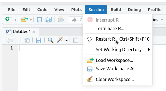
2. If the
Environmenttab isn’t empty click on the broom icon to clear it: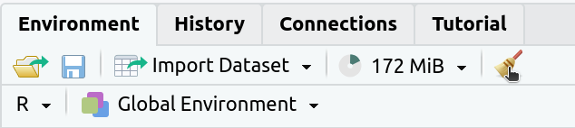
The
Environmenttab should now say “Environment Is Empty”: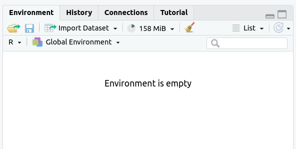
3. Rerun your entire homework assignment using “Source with Echo” to make sure it runs from start to finish and produces the expected results.
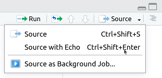
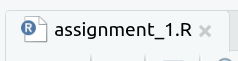
4. Make sure that you saved your code with the name
assignmentsomewhere in the file name. You should see the file in theFilestab and the name of the file should be black (not red with an*in the tab at the top of the text editor):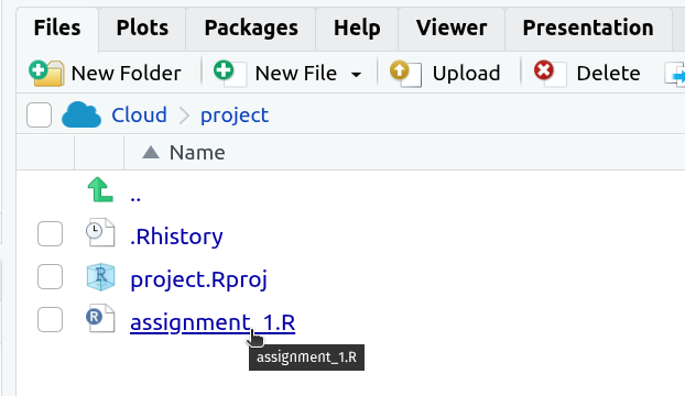
5. Make sure that your code will run on other computers
- No
setwd()(use RStudio Projects instead) - Use
/not\for paths
- No
M'Baïki Data Challenge (Challenge - optional)
A long-term study near M’Baïki in the Central African Republic has been monitoring tropical forest recovery from disturbance for 40 years.
Use the data on yearly tree measurements (in mbaiki_measures.csv), information on the individual trees (in mbaiki_trees.csv), and the names of the species in the forest (in mbaiki_species.csv) to answer the following questions (if isn’t in your working directory download it).
- Create a new data frame that contains the following information for each unique tree (each tree has a unique
id_tree): Theid_tree, the net growth (total change in diameter from the first year a tree is measured to the last year a tree is measured), the time period of sampling in years (number of years between the first and last measurement), and the growth rate (the net growth divided by the time period of sampling). Only include observations while the tree was alive in these calculations. - Starting with the data frame you created in (1) create a new data frame that contains the following information on the average growth rate of trees in each species in each subplot: The ID of the subplot, the scientific name of the species, the mean growth rate of all of the trees of that species in that subplot, and the sample size used to estimate the mean (i.e., the number of trees of that species in that subplot). Make sure the resulting data frame is not grouped.
Find out more about this dataset by accessing the full dataset or reading the associated paper: Bénédet, F., Gourlet-Fleury, S., Allah-Barem, F. et al. 2024. 40 years of forest dynamics and tree demography in an intact tropical forest at M’Baïki in central Africa. Sci Data 11, 734.
Expected outputs for M'Baïki Data Challenge- Create a new data frame that contains the following information for each unique tree (each tree has a unique