Learning Objectives
Following this assignment students should be able to:
- install and load an R package
- understand the data manipulation functions of
dplyr- execute a simple import and analyze data scenario
Reading
Readings
Optional Resources:
- Data Analysis and Visualization in R for Ecologists - Working with data
- dplyr vignette
- Mapping between dplyr and base R
Lecture Notes
Setup
install.packages(c('dplyr', 'readr', 'tidyr'))
download.file("https://ndownloader.figshare.com/files/2292172",
              "surveys.csv")
download.file("https://ndownloader.figshare.com/files/3299474",
              "plots.csv")
download.file("https://ndownloader.figshare.com/files/3299483",
              "species.csv")
download.file("https://www.datacarpentry.org/semester-biology/data/shrub-volume-data.csv",
              "shrub-volume-data.csv")
download.file("https://www.datacarpentry.org/semester-biology/data/penguins.csv",
              "penguins.csv")
Lecture Notes
- Working with Tabular Data (in dplyr)
- Basic Code Execution Order
- Combining Data Manipulations
- AI - Introduction and Basic Prompting
Place this code at the start of the assignment to load all the required packages.
library(dplyr)
Exercises
Shrub Volume Data Basics Select (5 pts)
Dr. Morales is interested in studying the factors controlling the size and carbon storage of shrubs. She has conducted an experiment looking at the effect of three different treatments on shrub volume at four different locations. She has placed the data file on the web for you to download:
If the file
shrub-volume-data.csvis not already in your working directory (it probably is if you’re taking this class using Posit Cloud) then download it into your working directory.Get familiar with the data by importing it using
read_csv()and usedplyrto complete the following tasks.- Select the data from the length column (using
select). - Select the data from the site and experiment columns (using
select). - Select the data from the experiment, length, width, and height columns
- Select the data from the length column (using
Penguin Data Basics Select (5 pts)
If the file
penguins.csvis not already in your working directory then download it into your working directory.Load the data using
read_csv()and usedplyrto complete the following tasks.- Select the data from the
speciescolumn. - Select the data from the
islandandyear. - Select the data from the
species,bill_length_mm,bill_depth_mm, andbody_mass_gcolumns.
- Select the data from the
Shrub Volume Data Basics Mutate (5 pts)
Dr. Morales is interested in studying the factors controlling the size and carbon storage of shrubs. She has conducted an experiment looking at the effect of three different treatments on shrub volume at four different locations. She has placed the data file on the web for you to download:
If the file
shrub-volume-data.csvis not already in your working directory (it probably is if you’re taking this class using Posit Cloud) then download it into your working directory.Get familiar with the data by importing it using
read_csv()and usedplyrto complete the following tasks.- Sort the data by length (using
arrange). - Add a new column named
areacontaining the area of the shrub (length x width) (usingmutate). - Add a new column named
volumecontaining the volume of the shrub (length x width x height) (usingmutate).
- Sort the data by length (using
Penguin Data Basics Mutate (5 pts)
If the file
penguins.csvis not already in your working directory then download it into your working directory.Load the data using
read_csv()and usedplyrto complete the following tasks.- Add a new column named
bill_ratiocontaining the ratio of the penguin’s bill length to its bill depth (bill length / bill depth). - Sort the data by body mass.
- Add a new column named
Shrub Volume Data Basics Filter (5 pts)
Dr. Morales is interested in studying the factors controlling the size and carbon storage of shrubs. She has conducted an experiment looking at the effect of three different treatments on shrub volume at four different locations. She has placed the data file on the web for you to download:
If the file
shrub-volume-data.csvis not already in your working directory (it probably is if you’re taking this class using Posit Cloud) then download it into your working directory.Get familiar with the data by importing it using
read_csv()and usedplyrto complete the following tasks.- Filter the data to include only plants with heights greater than 5 (using
filter). - Filter the data to include only plants with heights greater than 4 and widths greater than 2 (using
,or&to include two conditions). - Filter the data to include only plants from Experiment 1 or Experiment 3 (using
%in%).
- Filter the data to include only plants with heights greater than 5 (using
Penguin Data Basics Filter (5 pts)
If the file
penguins.csvis not already in your working directory then download it into your working directory.Load the data using
read_csv()and usedplyrto complete the following tasks.- Filter the data to include only penguins with flippers longer than 210 mm.
- Filter the data to include only penguins with flippers longer than 210 mm and body masses greater than 5000 g.
- Filter the data to include only penguins from the Dream or Torgersen islands.
Shrub Volume Data Basics Filter NA (5 pts)
Dr. Morales is interested in studying the factors controlling the size and carbon storage of shrubs. She has conducted an experiment looking at the effect of three different treatments on shrub volume at four different locations. She has placed the data file on the web for you to download:
If the file
shrub-volume-data.csvis not already in your working directory (it probably is if you’re taking this class using Posit Cloud) then download it into your working directory.Get familiar with the data by importing it using
read_csv()and usedplyrto complete the following tasks.- Remove rows with null values in the
heightcolumn (usingdrop_na). - Remove rows with null values in the
heightandwidthcolumns (usingdrop_na).
- Remove rows with null values in the
Penguin Data Basics Filter NA (5 pts)
If the file
penguins.csvis not already in your working directory then download it into your working directory.Load the data using
read_csv()and usedplyrto complete the following tasks.- Remove rows with null values in the
body_mass_gcolumn. - Remove rows with null values in the
sexcolumn. - Create a new data frame called
penguin_massesthat includes all of the original data with no null body masses and a new column containing the body mass in kilograms (body mass in grams / 1000).
- Remove rows with null values in the
Code Shuffle (5 pts)
We are interested in understanding the monthly variation in precipitation in Gainesville, FL. We’ll use some data from the NOAA National Climatic Data Center. Each row of the data is a year (from 1961-2013) and each column is a month (January - December).
Rearrange the following program so that it:
- Loads the readr package
- Imports the data from the web into a data frame
- Calculates the mean precipitation (ppt) in each month across years
- Plots the monthly averages as a simple line plot
Finally, add a comment above the code that describes what it does. The comment character in R is
#.It’s OK if you don’t know exactly how the details of the program work at this point, you just need to figure out the right order of the lines based on when variables are defined and when they are used.
Expected outputs for Code Shuffleplot(monthly_mean_ppt, type = "l", xlab = "Month", ylab = "Mean Precipitation") monthly_mean_ppt <- colMeans(ppt_data) library(readr) ppt_data <- read_csv("https://datacarpentry.org/semester-biology/data/gainesville-precip.csv", col_names = FALSE)Bird Banding (10 pts)
The number of birds banded at a series of sampling sites has been counted by your field crew and entered into the following vector. Counts are entered in order and sites are numbered starting at one. Cut and paste the vector into your assignment and then answer the following questions by using code and printing the result to the screen. Some R functions that will come in handy include
length(),max(),min(),sum(), andmean().number_of_birds <- c(28, 32, 1, 0, 10, 22, 30, 19, 145, 27, 36, 25, 9, 38, 21, 12, 122, 87, 36, 3, 0, 5, 55, 62, 98, 32, 900, 33, 14, 39, 56, 81, 29, 38, 1, 0, 143, 37, 98, 77, 92, 83, 34, 98, 40, 45, 51, 17, 22, 37, 48, 38, 91, 73, 54, 46, 102, 273, 600, 10, 11)- How many sites are there?
- How many birds were counted at site 42?
- What is the total number of birds counted across all of the sites?
- What is the smallest number of birds counted?
- What is the largest number of birds counted?
- What is the average number of birds seen at a site?
- How many birds were counted at the last site? Have the computer choose the last site automatically in some way, not by manually entering its position. Do you know a function that will give you the position of the last value? (since positions start at 1 the position of the last value in a vector is the same as its length).
Portal Data Manipulation (15 pts)
If the file
surveys.csvis not already in your working directory then download a copy.Load the file into R using
read_csv().Do not use pipes for this exercise.
- Use
select()andarrange()to create a new data frame with just theyear,month,day, andplot_idcolumns with the rows sorted byplot_id. - Use
mutate(),select(), anddrop_na()to create a new data frame with theyear,species_id, and weight in kilograms of each individual, with no null weights. The weight in the table is given in grams so you will need to create a new column for weight in kilograms by dividing the weight column by 1000. - Use
filter()andselect()to get theyear,month,day, andspecies_idcolumns for all of the rows in the data frame where species_id is SH. - Use
select(),filter(), andarrange()to produce a data frame withplot_id,species_id,weight, andhindfoot_length, where the species is"PB"or"PP"andweightis less than 40. Exclude NA values for bothweightandhindfoot_length. Sort the table byweight.
- Use
Portal Data Manipulation Pipes (20 pts)
If the file
surveys.csvis not already in your working directory then download a copy.Load the file into R using
read_csv().Use pipes (
|>) to combine the following operations to manipulate the data.- Use
select()andarrange()to create a new data frame with just theyear,month,day,species_id, andplot_idcolumns with the rows sorted byspecies_id. - Use
mutate(),select(), anddrop_na()to create a new data frame with theyear,species_id, andhindfoot_lengthin cm of each individual, with no null hindfoot lengths. The hindfoot length in the table is given in mm so you will need to create a new column for hindfoot length in cm by dividing thehindfoot_lengthcolumn by 10. - Use
filter()andselect()to get theyear,month,day, andspecies_idcolumns for all of the rows in the data frame where species_id is"OT". - Use
select(),filter(), andarrange()to produce a data frame withplot_id,species_id,weight, andhindfoot_length, where the species is"DM"or"DS"andhindfoot_lengthis greater than 35. Exclude NA values for bothweightandhindfoot_length. Sort the result byhindfoot_length.
- Use
Check That Your Code Runs (10 pts)
Sometimes you think you’re code runs, but it only actually works because of something else you did previously. To make sure it actually runs you should save your work and then run it in a clean environment.
Follow these steps in RStudio to make sure your code really runs:
1. Restart R (see above) by clicking
Sessionin the menu bar and selectingRestart R: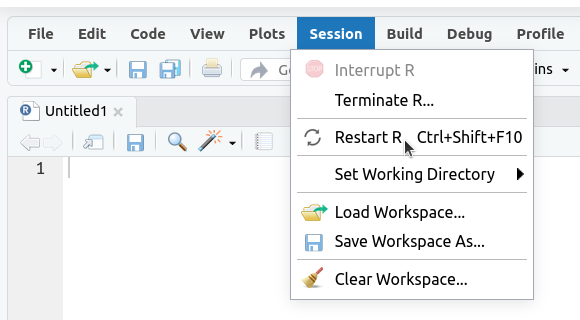
2. If the
Environmenttab isn’t empty click on the broom icon to clear it: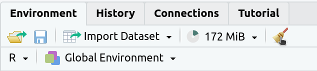
The
Environmenttab should now say “Environment Is Empty”: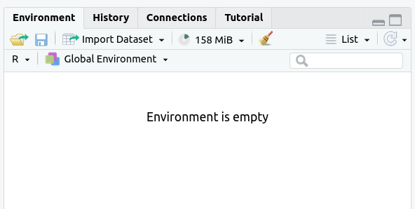
3. Rerun your entire homework assignment using “Source with Echo” to make sure it runs from start to finish and produces the expected results.
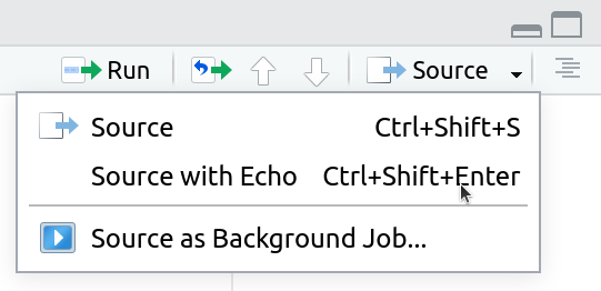
4. Make sure that you saved your code with the name
assignmentsomewhere in the file name. You should see the file in theFilestab and the name of the file should be black (not red with an*in the tab at the top of the text editor):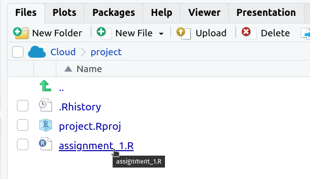
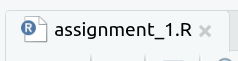
5. Make sure that your code will run on other computers
- No
setwd()(use RStudio Projects instead) - Use
/not\for paths
- No
Portal Data Challenge (Challenge - optional)
If the file
surveys.csvis not already in your working directory then download a copy.Develop a data manipulation pipeline for the Portal
Expected outputs for Portal Data Challengesurveystable that produces a table of data for only the three Dipodomys species (DM,DO,DS). The species IDs should be presented as lower case, not upper case. The table should contain information on the date, the species ID, the weight and hindfoot length. The data should not include null values for either weight or hindfoot length. The table should be sorted first by the species (so that each species is grouped together) and then by weight, with the largest weights at the top.