Learning Objectives
Following this assignment students should be able to:
- use, modify, and write custom functions
- use the output of one function as the input of another
Reading
-
Topics
- Functions
-
Readings
Lecture Notes
Setup
install.packages(c('dplyr', 'ggplot2', 'readr', 'tidyr'))
download.file("https://ndownloader.figshare.com/files/2292172",
  "surveys.csv")
download.file("https://ndownloader.figshare.com/files/3299474",
  "plots.csv")
download.file("https://ndownloader.figshare.com/files/3299483",
  "species.csv")
Lecture Notes
Exercises
Writing Functions (15 pts)
1. Copy the following function (which converts weights in pounds to weights in grams) into your assignment and replace the
________with the variable names for the input and output.convert_pounds_to_grams <- function(________) { grams = 453.6 * pounds return(________) }Use the function to calculate how many grams there are in 3.75 pounds.
2. Copy the following function (which converts temperatures in Fahrenheit to temperatures in Celsius) into your assignment and replace the
________with the needed commands and variable names so that the function returns the calculated value for Celsius.convert_fahrenheit_to_celsius <- ________(________) { celsius = (fahrenheit - 32) * 5 / 9 ________(________) }Use the function to calculate the temperature in Celsius if the temperature in Fahrenheit is 80°F.
3. Write a function named
doublethat takes a number as input and outputs that number multiplied by 2. Run it with an input of 512.4. Write a function named
Expected outputs for Writing Functionspredictionthat takes three arguments,x,a, andb, and returnsyusingy = a + b * x(like a prediction from a simple linear model). Run it withx= 12,a= 6, andb= 0.8.Use and Modify (15 pts)
The length of an organism is typically strongly correlated with its body mass. This is useful because it allows us to estimate the mass of an organism even if we only know its length. This relationship generally takes the form:
mass = a * lengthb
Where the parameters
aandbvary among groups. This allometric approach is regularly used to estimate the mass of dinosaurs since we cannot weigh something that is only preserved as bones.The following function estimates the mass of an organism in kg based on its length in meters for a particular set of parameter values, those for Theropoda (where
ahas been estimated as0.73andbhas been estimated as3.63; Seebacher 2001).get_mass_from_length_theropoda <- function(length){ mass <- 0.73 * length ^ 3.63 return(mass) }- Use this function to print out the mass of a Theropoda that is 16 m long based on its reassembled skeleton.
- Create a new version of this function called
get_mass_from_length()that takeslength,aandbas arguments and uses the following code to estimate the massmass <- a * length ^ b. Use this function to estimate the mass of a Sauropoda (a = 214.44,b = 1.46) that is 26 m long.
Writing Functions 2 (15 pts)
1. Copy the following function (which converts weights in pounds to weights in grams and rounds them) into your assignment. Replace the
________with the variable names for the input and output. Replace__with a number so that by default the function will round the output to one decimal place.convert_pounds_to_grams <- function(________, numdigits = __) { grams <- 453.6 * pounds rounded <- round(grams, digits = numdigits) return(________) }Use the function to calculate how many grams there are in 4.3 pounds using the default for the number of decimal places.
2. Write a function called
get_height_from_weightthat takes three arguments,weight,a, andb, and returns an estimate ofheightusingheight = a * weight ^ b(a prediction from a power model). Give it default arguments ofa= 12 andb= 0.38. There should be no default value forweight. Use the default argument values (by passing only the value ofweightto the function) to calculateheightwhenweight= 42.3. Call the function from (2) setting
weightto 42,ato 6, andbto 0.5.4. The function in (2) assumes that the weight is provided in grams. Use the functions from (1) and (2) in combination to estimate the height for an animal that weighs 2 pounds using the default value for
Expected outputs for Writing Functions 2a, but changing the value forbto 0.32.Default Arguments (15 pts)
The following function estimates the mass of an organism in kg based on its length in meters and a set of parameter values. For some types of dinosaurs we don’t have specific values of
aandb, so we have to use general values that can be applied to a number of different species.get_mass_from_length_theropoda <- function(length, a, b){ mass <- a * length ^ b return(mass) }Rewrite this function so that its arguments have default values of
a = 39.9andb = 2.6(the average values from Seebacher 2001).- Use this function to estimate the mass of a Sauropoda (
a = 214.44,b = 1.46) that is 22 m long (by settingaandbwhen calling the function). - Use this function to estimate the mass of a dinosaur from an unknown taxonomic group that is 16m long.
Only pass the function
length, notaandb, so that the default values are used.
- Use this function to estimate the mass of a Sauropoda (
Combining Functions (15 pts)
Write two functions:
- One called
get_mass_from_length()that takeslength(in m),aandbas arguments, has the following default argumentsa = 39.9andb = 2.6, uses the following code to estimate the mass (in kg)mass <- a * length ^ b, and returns it. (This function is the answer to the Default Arguments exercise, so feel free to copy over your answer if you’ve done that exercise). - One called
convert_kg_to_poundsthat converts kilograms into pounds (pounds = 2.205 * kg)
-
Use these two functions (each function should be called separately) to estimate the weight, in pounds, of a 12 m long Stegosaurus with
a = 10.95andb = 2.64(The estimatedaandbvalues for Stegosauria from Seebacher 2001). -
Use these two functions (each function should be called separately) to estimate the weight, in pounds, of a 4 m long dinosaur using the default parameters.
- One called
Writing Tidyverse Functions (15 pts)
1. Copy the following vectors into R and combine them into a data frame named
count_datawith columns namedstate,count,area, andsite.state_vector <- c("FL", "FL", "FL", "FL", "GA", "GA", "GA", "GA", "SC", "SC", "SC", "SC") site_vector <- c("A", "B", "C", "D", "A", "B", "C", "D", "A", "B", "C", "D") count_vector <- c(9, 16, 3, 10, 2, 26, 5, 8, 17, 8, 2, 6) area_vector <- c(3, 5, 1.9, 2.7, 2, 2.6, 6.2, 4.5, 8, 4, 1, 3)2. Write a function that takes two arguments: 1) a data frame with a
countcolumn and anareacolumn; and 2) a column in that data frame to color the points by. Have the function make a plot withareaon the x-axis andcounton the y-axis and the points colored by the column you provided as an argument. Set the size of the points to 3. Use the function to make a scatter plot of count as a function of area for thecount_datadata frame with the points colored by thestatecolumn.3. Use the function from (2) to make a scatter plot of count as a function of area for the
Expected outputs for Writing Tidyverse Functionscount_datadata frame with the points colored by thesitecolumn.Check That Your Code Runs (10 pts)
Sometimes you think you’re code runs, but it only actually works because of something else you did previously. To make sure it actually runs you should save your work and then run it in a clean environment.
Follow these steps in RStudio to make sure your code really runs:
1. Restart R (see above) by clicking
Sessionin the menu bar and selectingRestart R: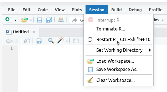
2. If the
Environmenttab isn’t empty click on the broom icon to clear it:
The
Environmenttab should now say “Environment Is Empty”: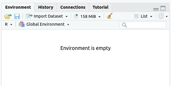
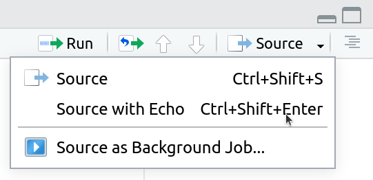
3. Rerun your entire homework assignment using “Source with Echo” to make sure it runs from start to finish and produces the expected results.
4. Make sure that you saved your code with the name
assignmentsomewhere in the file name. You should see the file in theFilestab and the name of the file should be black (not red with an*in the tab at the top of the text editor):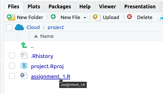

5. Make sure that your code will run on other computers
- No
setwd()(use RStudio Projects instead) - Use
/not\for paths
- No
Portal Species Time-Series Challenge (Challenge - optional)
If surveys.csv, species.csv, and plots.csv are not available in your workspace download them:
Write a function that:
- Takes four arguments - 1) a data frame (where each row is one individual and there is a
genusand aspeciescolumn); 2) atimeargument that provides the column to use for plotting time (e.g.,year); 3) agenus_nameargument for choosing which genus to plot; and 4) aspecies_nameargument for choosing which species to plot. - Makes a plot using
ggplot2with the time on the x-axis, thecountof the number of individuals (i.e., the number of rows) on the y-axis, and only plotting data for the species indicated by thegenus_nameandspecies_namearguments. The plot should display the data as blue points (with size = 2) connected by blue lines (with linewidth = 1). Make y-axis labelNumber of Individuals.
- Use your function, and the data in
surveys.csvandspecies.csv, to plot the time-series fortime=year,genus_name="Dipodomys"andspecies_name="merriami" - Use your function, and the data in
surveys.csvandspecies.csv, to plot the time-series fortime=month,genus_name="Chaetodipus"andspecies_name="penicillatus"(this plot will show the average seasonal pattern of Chaetodipus penicillatus abundances) - Use your function, and the data from
plots.csv,surveys.csvandspecies.csv, anddplyrto plot the time-series fortime=year,genus_name="Chaetodipus"andspecies_name="baileyi"only on the"Control"plots.
- Takes four arguments - 1) a data frame (where each row is one individual and there is a