Spatial Data Raster

Remember to download and put into data subdirectory:

• LiDAR rasters and plot locations

Load the following into browser window:

• Raster description
• Canopy Height Model picture

Introduction to raster data

• There are two common types of spatial data, raster and vector
• Raster data stores data that is continous across space
• Like climate variables, satellite imagery, and elevation
• It is stored in a gridded format

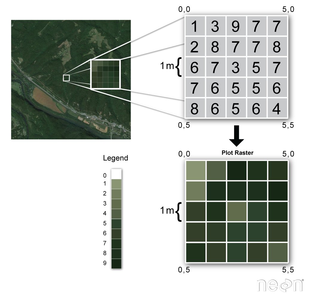
• In the grid each pixel contains a value
• So it is basically a matrix of numbers of one value at each position in the matrix
• So for elevation we would have a matrix of heights above sea level

Importing and exploring

• We import raster data using the read_stars() function from the stars package
• We’ll start by importing some elevation data collected from an airplane using an instrument called LIDAR
• One of the values that LIDAR can generate is a Digital Terrain Model or DTM, which is the elevation of the ground

library(stars)
dtm_harv <- read_stars("data/harv/harv_dtmcrop.tif")

• Looking at this object provides information on the data it contains

dtm_harv

• This is “metadata” or “data about “data”
• It is is important because it provides the context of spatial data this raster matrix so that R knows how to work with it
  • refsys
  • units
  • min, max, mean

Plotting spatial data with ggplot

• Spatial data can be plotted using either base R or ggplot
• We’ll use ggplot since that’s the data visualization tool we’re using for this course

• Useful for making nice maps combined with other figures

• There is a special geom for plotting stars raster data geom_stars
• Since it is raster data it doesn’t require an aesthetic

library(ggplot2)

ggplot() +
  geom_stars(data = dtm_harv)

• For spatial data we’re going to put the data in the geom calls instead of ggplot() because we are often trying to combine data of different types from different objects into a single map

• We can change the color ramp by using scale functions
• This is equivalent to when we used scale to change the axes, but now we’re changing the color ramp instead
• One good color ramp is “viridis”
• To use this color ramp we add `scale_fill_viridis_c() to our ggplot object
• We use fill because we are coloring the inside of each raster pixel (like the inside of a bar plot or histogram)
• The _c at the end indicates that it is a “continuous” scale

ggplot() +
  geom_stars(data = dtm_harv) +
  scale_fill_viridis_c()

• If we had discrete data, e.g., on soil types, we would use _d instead

Do Task 1 of Canopy Height from Space.