Data Analysis and Visualization with Python for Social Scientists *alpha*: All in One View

Last updated on 2023-05-04 | Edit this page

Overview

Questions

Why learn Python?
What are Jupyter notebooks?

Objectives

Examine the Python interpreter
Recognize the advantage of using the Python programming language
Understand the concept and benefits of using notebooks for coding

Introducing the Python programming language

Python is a general purpose programming language. It is an interpreted language, which makes it suitable for rapid development and prototyping of programming segments or complete small programs.

Python’s main advantages:

Open source software, supported by Python Software Foundation
Available on all major platforms (Windows, macOS, Linux)
It is a good language for new programmers to learn due to its straightforward, object-oriented style
It is well-structured, which aids readability
It is extensible (i.e. modifiable) and is supported by a large community who provide a comprehensive range of 3rd party packages

Interpreted vs. compiled languages

In any programming language, the code must be translated into “machine code” before running it. It is the machine code which is executed and produces results. In a language like C++ your code is translated into machine code and stored in a separate file, in a process referred to as compiling the code. You then execute the machine code from the file as a separate step. This is efficient if you intend to run the same machine code many times as you only have to compile it once and it is very fast to run the compiled machine code.

On the other hand, if you are experimenting, then your code will change often and you would have to compile it again every time before the machine can execute it. This is where interpreted languages have the advantage. You don’t need a complete compiled program to “run” what has been written so far and see the results. This rapid prototyping is helped further by use of a system called REPL.

REPL

REPL is an acronym which stands for Read, Evaluate, Print and Loop.

REPL allows you to write single statements of code, have them executed, and if there are any results to show, they are displayed and then the interpreter loops back to the beginning and waits for the next program statement.

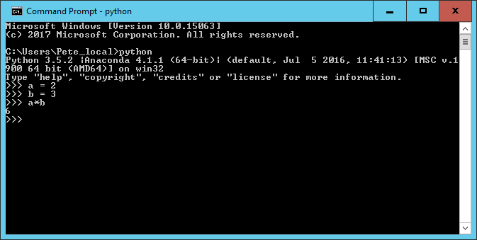
In the example above, two variables a and b have been created, assigned to values 2 and 3, and then multiplied together.

Every time you press Return, the line is interpreted. The assignment statements don’t produce any output so you get only the standard >>> prompt.

For the a*b statement (it is more of an expression than a statement), because the result is not being assigned to a variable, the REPL displays the result of the calculation on screen and then waits for the next input.

The REPL system makes it very easy to try out small chunks of code.

You are not restricted to single line statements. If the Python interpreter decides that what you have written on a line cannot be a complete statement it will give you a continuation prompt of ... until you complete the statement.

Introducing Jupyter notebooks

Jupyter originates from IPython, an effort to make Python development more interactive. Since its inception, the scope of the project has expanded to include Julia, Python, and R, so the name was changed to “Jupyter” as a reference to these core languages. Today, Jupyter supports even more languages, but we will be using it only for Python code. Specifically, we will be using Jupyter notebooks, which allows us to easily take notes about our analysis and view plots within the same document where we code. This facilitates sharing and reproducibility of analyses, and the notebook interface is easily accessible through any web browser. Jupyter notebooks are started from the terminal using

BASH

$ jupyter notebook

Your browser should start automatically and look something like this:

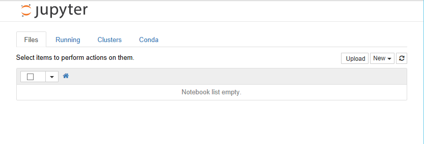
When you create a notebook from the New option, the new notebook will be displayed in a new browser tab and look like this.

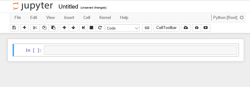
Initially the notebook has no name other than ‘Untitled’. If you click on ‘Untitled’ you will be given the option of changing the name to whatever you want.

The notebook is divided into cells. Initially there will be a single input cell marked by In [ ]:.

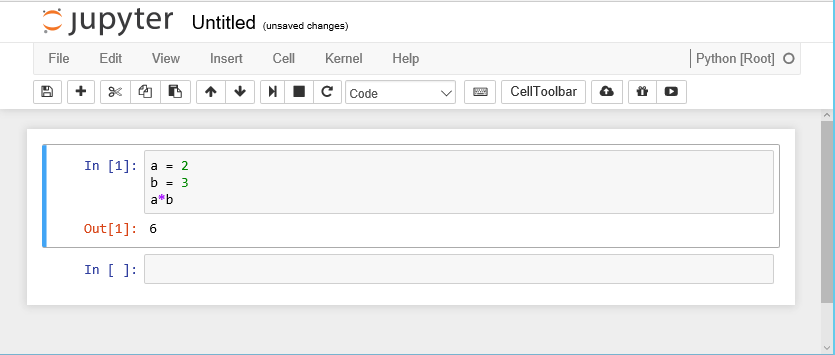
You can type Python code directly into the cell. You can split the code across several lines as needed. Unlike the REPL we looked at before, the code is not interpreted line by line. To interpret the code in a cell, you can click the Run button in the toolbar or from the Cell menu option, or use keyboard shortcuts (e.g., Shift+Return). All of the code in that cell will then be executed.

The results are shown in a separate Out [1]: cell immediately below. A new input cell (In [ ]:) is created for you automatically.

When a cell is run, it is given a number along with the corresponding output cell. If you have a notebook with many cells in it you can run the cells in any order and also run the same cell many times. The number on the left hand side of the input cells increments, so you can always tell the order in which they were run. For example, a cell marked In [5]: was the fifth cell run in the sequence.

Although there is an option to do so on the toolbar, you do not have to manually save the notebook. This is done automatically by the Jupyter system.

Not only are the contents of the In [ ]: cells saved, but so are the Out [ ]: cells. This allows you to create complete documents with both your code and the output of the code in a single place. You can also change the cell type from Python code to Markdown using the Cell > Cell Type option. Markdown is a simple formatting system which allows you to create documentation for your code, again all within the same notebook structure.

The notebook itself is stored as specially-formatted text file with an .ipynb extension. These files can be opened and run by others with Jupyter installed. This allows you to share your code inputs, outputs, and Markdown documentation with others. You can also export the notebook to HTML, PDF, and many other formats to make sharing even easier.

Key Points

Python is an interpreted language
The REPL (Read-Eval-Print loop) allows rapid development and testing of code segments
Jupyter notebooks builds on the REPL concepts and allow code results and documentation to be maintained together and shared
Jupyter notebooks is a complete IDE (Integrated Development Environment)

Content from Python basics

Last updated on 2023-05-04 | Edit this page

Overview

Questions

How do I assign values to variables?
How do I do arithmetic?
What is a built-in function?
How do I see results?
What data types are supported in Python?

Objectives

Create different cell types and show/hide output in Jupyter
Create variables and assign values to them
Check the type of a variable
Perform simple arithmetic operations
Specify parameters when using built-in functions
Get help for built-in functions and other aspects of Python
Define native data types in Python
Convert from one data type to another

Using the Jupyter environment

New cells

From the insert menu item you can insert a new cell anywhere in the notebook either above or below the current cell. You can also use the + button on the toolbar to insert a new cell below.

Change cell type

By default new cells are created as code cells. From the cell menu item you can change the type of a cell from code to Markdown. Markdown is a markup language for formatting text, it has much of the power of HTML, but is specifically designed to be human-readable as well. You can use Markdown cells to insert formatted textual explanation and analysis into your notebook. For more information about Markdown, check out these resources:

Hiding output

When you run cells of code the output is displayed immediately below the cell. In general this is convenient. The output is associated with the cell that produced it and remains a part of the notebook. So if you copy or move the notebook the output stays with the code.

However lots of output can make the notebook look cluttered and more difficult to move around. So there is an option available from the cell menu item to ‘toggle’ or ‘clear’ the output associated either with an individual cell or all cells in the notebook.

Creating variables and assigning values

Variables and Types

In Python variables are created when you first assign values to them.

PYTHON

a = 2
b = 3.142

All variables have a data type associated with them. The data type is an indication of the type of data contained in a variable. If you want to know the type of a variable you can use the built-in type() function.

PYTHON

print(type(a))
print(type(b))
s = "Hello World"
print(type(s))

OUTPUT

<class 'int'>
<class 'float'>
<class 'str'>

There are many more data types available, a full list is available in the Python documentation. We will be looking a few of them later on.

Arithmetic operations

For now we will stick with the numeric types and do some arithmetic.

All of the usual arithmetic operators are available.

In the examples below we also introduce the Python comment symbol #. Anything to the right of the # symbol is treated as a comment. To a large extent using Markdown cells in a notebook reduces the need for comments in the code in a notebook, but occasionally they can be useful.

We also make use of the built-in print() function, which displays formatted text.

PYTHON

print("a =", a, "and b =" , b)
print(a + b)      # addition
print(a * b)      # multiplication
print(a - b)      # subtraction
print(a / b)      # division
print(b ** a)     # exponentiation
print(a % b)      # modulus - returns the remainder
print(2 * a % b)  # modulus - returns the remainder

OUTPUT

a = 2 and b = 3.142
5.1419999999999995
6.284
-1.142
0.6365372374283896
9.872164
2.0
0.8580000000000001

We need to use the print() function because by default only the last output from a cell is displayed in the output cell.

In our example above, we pass four different parameters to the first call of print(), each separated by a comma. A string "a = ", followed by the variable a, followed by the string "b = " and then the variable b.

The output is what you would probably have guessed at.

All of the other calls to print() are only passed a single parameter. Although it may look like 2 or 3, the expressions are evaluated first and it is only the single result which is seen as the parameter value and printed.

In the last expression a is multiplied by 2 and then the modulus of the result is taken. Had we wanted to calculate a % b and then multiply the result by two we could have done so by using brackets to make the order of calculation clear.

When we have more complex arithmetic expressions, we can use parentheses to be explicit about the order of evaluation:

PYTHON

print("a =", a, "and b =" , b)
print(a + 2*b)    # add a to two times b
print(a + (2*b))  # same thing but explicit about order of evaluation
print((a + b)*2)  # add a and b and then multiply by two

OUTPUT

a = 2 and b = 3.142
8.283999999999999
8.283999999999999
10.283999999999999

Arithmetic expressions can be arbitrarily complex, but remember people have to read and understand them as well.

Exercise

Create a new cell and paste into it the assignments to the variables a and b and the contents of the code cell above with all of the print statements. Remove all of the calls to the print function so you only have the expressions that were to be printed and run the code. What is returned?
Now remove all but the first line (with the 4 items in it) and run the cell again. How does this output differ from when we used the print function?
Practice assigning values to variables using as many different operators as you can think of.
Create some expressions to be evaluated using parentheses to enforce the order of mathematical operations that you require

Show me the solution

Only the last result is printed.
The 4 ‘items’ are printed by the REPL, but not in the same way as the print statement. The items in quotes are treated as separate strings, for the variables a and b the values are printed. All four items are treated as a ‘tuple’ which are shown in parentheses, a tuple is another data type in Python that allows you to group things together and treat as a unit. We can tell that it is a tuple because of the ()

A complete set of Python operators can be found in the official documentation . The documentation may appear a bit confusing as it initially talks about operators as functions whereas we generally use them as ‘in place’ operators. Section 10.3.1 provides a table which list all of the available operators, not all of which are relevant to basic arithmetic.

Using built-in functions

Python has a reasonable number of built-in functions. You can find a complete list in the official documentation.

Additional functions are provided by 3rd party packages which we will look at later on.

For any function, a common question to ask is: What parameters does this function take?

In order to answer this from Jupyter, you can type the function name and then type shift+tab and a pop-up window will provide you with various details about the function including the parameters.

Exercise

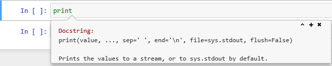
For the print() function find out what parameters can be provided

Show me the solution

Type ‘print’ into a code cell and then type shift+tab. The following pop-up should appear.

Getting Help for Python

You can get help on any Python function by using the help function. It takes a single parameter of the function name for which you want the help.

PYTHON

help(print)

OUTPUT

Help on built-in function print in module builtins:

print(...)
    print(value, ..., sep=' ', end='\n', file=sys.stdout, flush=False)

    Prints the values to a stream, or to sys.stdout by default.
    Optional keyword arguments:
    file:  a file-like object (stream); defaults to the current sys.stdout.
    sep:   string inserted between values, default a space.
    end:   string appended after the last value, default a newline.
    flush: whether to forcibly flush the stream.

There is a great deal of Python help and information as well as code examples available from the internet. One popular site is stackoverflow which specialises in providing programming help. They have dedicated forums not only for Python but also for many of the popular 3rd party Python packages. They also always provide code examples to illustrate answers to questions.

You can also get answers to your queries by simply inputting your question (or selected keywords) into any search engine.

A couple of things you may need to be wary of: There are currently 2 versions of Python in use, in most cases code examples will run in either but there are some exceptions. Secondly, some replies may assume a knowledge of Python beyond your own, making the answers difficult to follow. But for any given question there will be a whole range of suggested solutions so you can always move on to the next.

Data types and how Python uses them

Changing data types

The data type of a variable is assigned when you give a variable a value as we did above. If you re-assign the value of a variable, you can change the data type.

You can also explicitly change the type of a variable by casting it using an appropriate Python builtin function. In this example we have changed a string to a float.

PYTHON

a = "3.142"
print(type(a))
a = float(a)
print(type(a))

OUTPUT

<class 'str'>
<class 'float'>

Although you can always change an integer to a float, if you change a float to an integer then you can lose part of the value of the variable and you won’t get an error message.

PYTHON

a = 3.142
print(type(a))
a = 3
print(type(a))
a = a*1.0
print(type(a))
a = int(a)
print(type(a))
a = 3.142
a = int(a)
print(type(a))
print(a)

OUTPUT

<class 'float'>
<class 'int'>
<class 'float'>
<class 'int'>
<class 'int'>
3

In some circumstances explicitly converting a data type makes no sense; you cannot change a string with alphabetic characters into a number.

PYTHON

b = "Hello World"
print(type(b))

b = int(b)
print(type(b))

OUTPUT

<class 'str'>
---------------------------------------------------------------------------
ValueError                                Traceback (most recent call last)
<ipython-input-8-9f5f81a470f9> in <module>()
      2 print(type(b))
      3
----> 4 b = int(b)
      5 print(type(b))

ValueError: invalid literal for int() with base 10: 'Hello World'

Strings

A string is a simple data type which holds a sequence of characters.

Strings are placed in quotes when they are being assigned, but the quotes don’t count as part of the string value.

If you need to use quotes as part of your string you can arbitrarily use either single or double quotes to indicate the start and end of the string.

PYTHON

mystring = "Hello World"
print(mystring)

name = "Peter"
mystring = 'Hello ' + name + ' How are you?'
print(mystring)

name = "Peter"
mystring = 'Hello this is ' + name + "'s code"
print(mystring)

OUTPUT

Hello World
Hello Peter How are you?
Hello this is Peter's code

String functions

There are a variety of Python functions available for use with strings. In Python a string is an object. An object put simply is something which has data, in the case of our string it is the contents of the string and methods. methods is another way of saying functions.

Although methods and functions are very similar in practice, there is a difference in the way you call them.

One typical bit of information you might want to know about a string is its length for this we use the len() function. For almost anything else you might want to do with strings, there is a method.

PYTHON

mystring = "Hello World"
print(len(mystring))

OUTPUT

The official documentation says, ‘A method is a function that “belongs to” an object. In Python, the term method is not unique to class instances: other object types can have methods as well. For example, list objects have methods called append, insert, remove, sort, and so on.’.

If you want to see a list of all of the available methods for a string (or any other object) you can use the dir() function.

PYTHON

print(dir(mystring))

OUTPUT

['__add__', '__class__', '__contains__', '__delattr__', '__dir__', '__doc__', '__eq__', '__format__', '__ge__', '__getattribute__', '__getitem__', '__getnewargs__', '__gt__', '__hash__', '__init__', '__iter__', '__le__', '__len__', '__lt__', '__mod__', '__mul__', '__ne__', '__new__', '__reduce__', '__reduce_ex__', '__repr__', '__rmod__', '__rmul__', '__setattr__', '__sizeof__', '__str__', '__subclasshook__', 'capitalize', 'casefold', 'center', 'count', 'encode', 'endswith', 'expandtabs', 'find', 'format', 'format_map', 'index', 'isalnum', 'isalpha', 'isdecimal', 'isdigit', 'isidentifier', 'islower', 'isnumeric', 'isprintable', 'isspace', 'istitle', 'isupper', 'join', 'ljust', 'lower', 'lstrip', 'maketrans', 'partition', 'replace', 'rfind', 'rindex', 'rjust', 'rpartition', 'rsplit', 'rstrip', 'split', 'splitlines', 'startswith', 'strip', 'swapcase', 'title', 'translate', 'upper', 'zfill']

The methods starting with __ are special or magic methods which are not normally used.

Some examples of the methods are given below. We will use others when we start reading files.

PYTHON

myString = "The quick brown fox"

print(myString.startswith("The"))
print(myString.find("The"))        # notice that string positions start with 0 like all indexing in Python
print(myString.upper())            # The contents of myString is not changed, if you wanted an uppercase version
print(myString)                    # you would have to assign it to a new variable

OUTPUT

True
0
THE QUICK BROWN FOX
The quick brown fox

The methods starting with ‘is…’ return a boolean value of either True or False

PYTHON

print(myString.isalpha())

OUTPUT

False

the example above returns False because the space character is not considered to be an Alphanumeric value.

In the example below, we can use the replace() method to remove the spaces and then check to see if the result isalpha chaining method in this way is quite common. The actions take place in a left to right manner. You can always avoid using chaining by using intermediary variables.

PYTHON

print(myString.replace(" ","").isalpha())

OUTPUT

True

For example, the following is equivalent to the above

PYTHON

mystring_clean = myString.replace(" ","")
print(mystring_clean.isalpha())

OUTPUT

True

If you need to refer to a specific element (character) in a string, you can do so by specifying the index of the character in [] you can also use indexing to select a substring of the string. In Python, indexes begin with 0 (for a visual, please see Strings and Character Data in Python: String Indexing or 9.4. Index Operator: Working with the Characters of a String).

PYTHON

myString = "The quick brown fox"

print(myString[0])
print(myString[12])
print(myString[18])

print(myString[0:3])
print(myString[0:])        # from index 0 to the end
print(myString[:9])        # from the beginning to one before index 9
print(myString[4:9])

OUTPUT

T
o
x
The
The quick brown fox
The quick
quick

Basic Python data types

So far we have seen three basic Python data types; Integer, Float and String. There is another basic data type; Boolean. Boolean variables can only have the values of either True or False. (Remember, Python is case-sensitive, so be careful of your spelling.) We can define variables to be of type boolean by setting their value accordingly. Boolean variables are a good way of coding anything that has a binary range (eg: yes/no), because it’s a type that computers know how to work with as we will see soon.

PYTHON

print(True)
print(False)
bool_val_t = True
print(type(bool_val_t))
print(bool_val_t)
bool_val_f = False
print(type(bool_val_f))
print(bool_val_f)

OUTPUT

True
False
<class 'bool'>
True
<class 'bool'>
False

Following two lines of code will generate error because Python is case-sensitive. We need to use ‘True’ instead of ‘true’ and ‘False’ instead of ‘false’.

PYTHON

print(true)
print(false)

OUTPUT

NameError   Traceback (most recent call last)
<ipython-input-115-b5911eeae48b> in <module>
----> 1 print(true)
      2 print(false)

NameError: name 'true' is not defined

We can also get values of Boolean type using comparison operators, basic ones in Python are == for “equal to”, != for “not equal to”, and >, <, or >=, <=.

PYTHON

print('hello' == 'HELLO')
print('hello' is 'hello')
print(3 != 77)
print(1 < 2)
print('four' > 'three')

OUTPUT

False
True
True
True
False

Exercise

Imagine you are considering different ways of representing a boolean value in your data set and you need to see how python will behave based on the different choices. Fill in the blanks using the built in functions we’ve seen so far in following code excerpt to test how Python interprets text. Write some notes for your research team on how to code True and False as they record the variable.

PYTHON

bool_val1 = 'TRUE'
print('read as type ',___(bool_val1))
print('value when cast to bool',___(bool_val1))

bool_val2 = 'FALSE'
print('read as type ',___(bool_val2))
print('value when cast to bool',___(bool_val2))

bool_val3 = 1
print('read as type ',___(bool_val3))
print('value when cast to bool',___(bool_val3))

bool_val4 = 0
print('read as type ',___(bool_val4))
print('value when cast to bool',___(bool_val4))

bool_val5 = -1
print('read as type ',___(bool_val5))
print('value when cast to bool',___(bool_val5))
print(bool(bool_val5))

Show me the solution

0 is represented as False and everything else, whether a number or string is counted as True

Structured data types

A structured data type is a data type which is made up of some combination of the base data types in a well defined but potentially arbitrarily complex way.

The list

A list is a set of values, of any type separated by commas and delimited by ‘[’ and ’]’

PYTHON

list1 = [6, 54, 89 ]
print(list1)
print(type(list1))

list2 = [3.142, 2.71828, 9.8 ]
print(list2)
print(type(list2))

myname = "Peter"
list3 = ["Hello", 'to', myname ]
print(list3)
myname = "Fred"
print(list3)
print(type(list3))

list4 = [6, 5.4, "numbers", True ]
print(list4)
print(type(list4))

OUTPUT

[6, 54, 89]
<class 'list'>
[3.142, 2.71828, 9.8]
<class 'list'>
['Hello', 'to', 'Peter']
['Hello', 'to', 'Peter']
<class 'list'>
[6, 5.4, 'numbers', True]
<class 'list'>

Exercise

We can index lists the same way we indexed strings before. Complete the code below and display the value of last_num_in_list which is 11 and values of odd_from_list which are 5 and 11 to check your work.

PYTHON

num_list = [4,5,6,11]

last_num_in_list = num_list[____]
print(last_num_in_list)

odd_from_list = [num_list[_____], ______]
print(odd_from_list)

Show me the solution

PYTHON

# Solution 1: Basic ways of solving this exercise using the core Python language
num_list = [4,5,6,11]

last_num_in_list = num_list[-1]
print(last_num_in_list)

odd_from_list = [num_list[1], num_list[3]]
print(odd_from_list)


# Solutions 2 and 3: Usually there are multiple ways of doing the same work. Once we learn about more advanced Python, we would be able to write more varieties codes like the followings to print the odd numbers:
import numpy as np
num_list = [4,5,6,11]

# Converting `num_list` list to an advanced data structure: `numpy array`
num_list_np_array = np.array(num_list)

# Filtering the elements which produces a remainder of `1`, after dividing by `2`
odd_from_list = num_list_np_array[num_list_np_array%2 == 1]
print(odd_from_list)

# or, Using a concept called `masking`
# Create a boolean list `is_odd` of the same length of `num_list` with `True` at the position of the odd values.
is_odd = [False, True, False, True]  # Mask array
odd_from_list = num_list_np_array[is_odd] # only the values at the position of `True` remain
print(odd_from_list)

The range function

In addition to explicitly creating lists as we have above it is very common to create and populate them automatically using the range() function in combination with the list() function

PYTHON

list5 = list(range(5))
print(list5)

OUTPUT

[0, 1, 2, 3, 4]

Unless told not to range() returns a sequence which starts at 0, counts up by 1 and ends 1 before the value of the provided parameter.

This can be a cause of confusion. range(5) above does indeed have 5 values, but rather than being 1,2,3,4,5 which you might naturally think, they are in fact 0,1,2,3,4. The range starts at 0 and stops one before the value of the single parameter we specified.

If you want different sequences, then you can modify the behavior of the range() function by using additional parameters.

PYTHON

list6 = list(range(1, 9))
print(list6)
list7 = list(range(2, 11, 2))
print(list7)

OUTPUT

[1, 2, 3, 4, 5, 6, 7, 8]
[2, 4, 6, 8, 10]

When you specify 3 parameters as we have for list(7); the first is start value, the second is one past the last value and the 3rd parameter is a step value by which to count. The step value can be negative

list7 produces the even numbers from 1 to 10.

Exercise

What is produced if you change the step value in list7 to -2 ? Is this what you expected?
Create a list using the range() function which contains the even number between 1 and 10 in reverse order ([10,8,6,4,2])

Show me the solution

PYTHON

list7 = list(range(2, 11, -2))
print(list7)

list8 = list(range(10, 1, -2))
print(list8)

list7 will print nothing because starting at 2 and incrementing by -2 is the wrong direction to 11.

The other main structured data type is the Dictionary. We will introduce this in a later episode when we look at JSON.

Key Points

The Jupyter environment can be used to write code segments and display results
Data types in Python are implicit based on variable values
Basic data types are Integer, Float, String and Boolean
Lists and Dictionaries are structured data types
Arithmetic uses standard arithmetic operators, precedence can be changed using brackets
Help is available for builtin functions using the help() function further help and code examples are available online
In Jupyter you can get help on function parameters using shift+tab
Many functions are in fact methods associated with specific object types

Content from Python control structures

Last updated on 2023-05-04 | Edit this page

Overview

Questions

What constructs are available for changing the flow of a program?
How can I repeat an action many times?
How can I perform the same task(s) on a set of items?

Objectives

Change program flow using available language constructs
Demonstrate how to execute a section of code a fixed number of times
Demonstrate how to conditionally execute a section of code
Demonstrate how to execute a section of code on a list of items

Programs are rarely linear

Most programs do not work by executing a simple sequential set of statements. The code is constructed so that decisions and different paths through the program can be taken based on changes in variable values.

To make this possible all programming language have a set of control structures which allow this to happen.

In this episode we are going to look at how we can create loops and branches in our Python code. Specifically we will look at three control structures, namely:

if..else..
while…
for …

The `if` statement and variants

The simple if statement allows the program to branch based on the evaluation of an expression

The basic format of the if statement is:

PYTHON

if expression :
    statement 1
    statement 2
    ...
    statement n

statement always executed

If the expression evaluates to True then the statements 1 to n will be executed followed by statement always executed . If the expression is False, only statement always executed is executed. Python knows which lines of code are related to the if statement by the indentation, no extra syntax is necessary.

Below are some examples:

PYTHON

print("\nExample 1\n")

value = 5
threshold= 4
print("value is", value, "threshold is ",threshold)
if value > threshold :
    print(value, "is bigger than ", threshold)

print("\nExample 2\n")


high_threshold = 6
print("value is", value, "new threshold is ",high_threshold)
if value > high_threshold :
    print(value , "is above ", high_threshold, "threshold")

print("\nExample 3\n")


mid_threshold = 5
print("value is", value, "final threshold is ",mid_threshold)
if value == mid_threshold :
    print("value, ", value, " and threshold,", mid_threshold, ", are equal")

OUTPUT

Example 1

value is 5 threshold is 4
5 is bigger than 4

Example 2

value is 5 new threshold is 6

Example 3

value is 5 final threshold is 5
value, 5, and threshold, 5, are equal

In the examples above there are three things to notice:

The colon : at the end of the if line. Leaving this out is a common error.
The indentation of the print statement. If you remembered the : on the line before, Jupyter (or any other Python IDE) will automatically do the indentation for you. All of the statements indented at this level are considered to be part of the if statement. This is a feature fairly unique to Python, that it cares about the indentation. If there is too much, or too little indentation, you will get an error.
The if statement is ended by removing the indent. There is no explicit end to the if statement as there is in many other programming languages

In the last example, notice that in Python the operator used to check equality is ==.

Exercise

Add another if statement to example 2 that will check if b is greater than or equal to a

Show me the solution

PYTHON

print("\nExample 2a\n")

a= 3
b= 4
print("a is", a, "b is",b)
if a > b :
    print(a, "is bigger than ", b)
if a <= b :
    print(b, "is bigger than or equal to ", a)

Instead of using two separate if statements to decide which is larger we can use the if ... else ... construct

PYTHON

# if ... else ...

value = 4
threshold = 5
print("value = ", value, "and threshold = ", threshold)

if value > threshold :
    print("above threshold")
else :
    print("below threshold")

OUTPUT

value = 4 and threshold = 5
below threshold

Exercise

Repeat above with different operators ‘<’ , ‘==’

A further extension of the if statement is the if ... elif ...else version.

The example below allows you to be more specific about the comparison of a and b.

PYTHON

# if ... elif ... else ... endIf

a = 5
b = 4
print("a = ", a, "and b = ", b)

if a > b :
    print(a, " is greater than ", b)
elif a == b :
    print(a, " equals ", b)
else :
    print(a, " is less than ", b)

OUTPUT

a = 5 and b = 4
5 is greater than 4

The overall structure is similar to the if ... else statement. There are three additional things to notice:

Each elif clause has its own test expression.
You can have as many elif clauses as you need
Execution of the whole statement stops after an elif expression is found to be True. Therefore the ordering of the elif clause can be significant.

The `while` loop

The while loop is used to repeatedly execute lines of code until some condition becomes False.

For the loop to terminate, there has to be something in the code which will potentially change the condition.

PYTHON

# while loop
n = 10
cur_sum = 0
# sum of n  numbers
i = 1
while  i <= n :
    cur_sum = cur_sum + i
    i = i + 1
print("The sum of the numbers from 1 to", n, "is ", cur_sum)

OUTPUT

The sum of the numbers from 1 to 10 is 55

Points to note:

The condition clause (i <= n) in the while statement can be anything which when evaluated would return a Boolean value of either True of False. Initially i has been set to 1 (before the start of the loop) and therefore the condition is True.
The clause can be made more complex by use of parentheses and and and or operators amongst others
The statements after the while clause are only executed if the condition evaluates as True.
Within the statements after the while clause there should be something which potentially will make the condition evaluate as False next time around. If not the loop will never end.
In this case the last statement in the loop changes the value of i which is part of the condition clause, so hopefully the loop will end.
We called our variable cur_sum and not sum because sum is a builtin function (try typing it in, notice the editor changes it to green). If we define sum = 0 now we can’t use the function sum in this Python session.

Exercise - Things that can go wrong with while loops

In the examples below, without running them try to decide why we will not get the required answer. Run each, one at a time, and then correct them. Remember that when the input next to a notebook cell is [*] your Python interpreter is still working.

PYTHON

# while loop - summing the numbers 1 to 10
n = 10
cur_sum = 0
# sum of n  numbers
i = 0
while  i <= n :
    i = i + 1
    cur_sum = cur_sum + i
    
print("The sum of the numbers from 1 to", n, "is ", cur_sum)

PYTHON

# while loop - summing the numbers 1 to 10
n = 10
cur_sum = 0
boolvalue = False
# sum of n  numbers
i = 0
while  i <= n and boolvalue:
    cur_sum = cur_sum + i
    i = i + 1
    
print("The sum of the numbers from 1 to", n, "is ", cur_sum)

PYTHON

# while loop - summing the numbers 1 to 10
n = 10
cur_sum = 0
# sum of n  numbers
i = 0
while  i != n :
    cur_sum = cur_sum + i
    i = i + 1

print("The sum of the numbers from 1 to", n, "is ", cur_sum)

PYTHON

# while loop - summing the numbers 1.1 to 9.9 i. steps of 1.1
n = 9.9
cur_sum = 0
# sum of n  numbers
i = 0
while  i != n :
    cur_sum = cur_sum + i
    i = i + 1.1
    print(i)
    
print("The sum of the numbers from 1.1 to", n, "is ", sum)

Show me the solution

Because i is incremented before the sum, you are summing 1 to 11.
The Boolean value is set to False the loop will never be executed.
When i does equal 10 the expression is False and the loop does not execute so we have only summed 1 to 9
Because you cannot guarantee the internal representation of Float, you should never try to compare them for equality. In this particular case the i never ‘equals’ n and so the loop never ends. - If you did try running this, you can stop it using Ctrl+c in a terminal or going to the kernel menu of a notebook and choosing interrupt.

The `for` loop

The for loop, like the while loop repeatedly executes a set of statements. The difference is that in the for loop we know in at the outset how often the statements in the loop will be executed. We don’t have to rely on a variable being changed within the looping statements.

The basic format of the for statement is

PYTHON

for variable_name in some_sequence :
    statement1
    statement2
    ...
    statementn

The key part of this is the some_sequence. The phrase used in the documentation is that it must be ‘iterable’. That means, you can count through the sequence, starting at the beginning and stopping at the end.

There are many examples of things which are iterable some of which we have already come across.

Lists are iterable - they don’t have to contain numbers, you iterate over the elements in the list.
The range() function
The characters in a string

PYTHON

print("\nExample 1\n")
for i in [1,2,3] :
    print(i)

print("\nExample 2\n")
for name in ["Tom", "Dick", "Harry"] :
    print(name)

print("\nExample 3\n")
for name in ["Tom", 42, 3.142] :
    print(name)

print("\nExample 4\n")
for i in range(3) :
    print(i)

print("\nExample 5\n")
for i in range(1,4) :
    print(i)

print("\nExample 6\n")
for i in range(2, 11, 2) :
    print(i)

print("\nExample 7\n")
for i in "ABCDE" :
    print(i)

print("\nExample 8\n")
longString = "The quick brown fox jumped over the lazy sleeping dog"
for word in longString.split() :
    print(word)

OUTPUT

Example 1

1
2
3

Example 2

Tom
Dick
Harry

Example 3

Tom
42
3.142

Example 4

0
1
2

Example 5

1
2
3

Example 6

2
4
6
8
10

Example 7

A
B
C
D
E

Example 8

The
quick
brown
fox
jumped
over
the
lazy
sleeping
dog

Exercise

Suppose that we have a string containing a set of 4 different types of values separated by , like this:

PYTHON

variablelist = "01/01/2010,34.5,Yellow,True"

Research the split() method and then rewrite example 8 from the for loop section above so that it prints the 4 components of variablelist

Show me the solution

PYTHON

# From the for loop section above
variablelist = "01/01/2010,34.5,Yellow,True"
for word in variablelist.split(",") :
    print(word)

The format of variablelist is very much like that of a record in a csv file. In later episodes we will see how we can extract these values and assign them to variables for further processing rather than printing them out.

Key Points

Most programs will require ‘Loops’ and ‘Branching’ constructs.
The if, elif, else statements allow for branching in code.
The for and while statements allow for looping through sections of code
The programmer must provide a condition to end a while loop.

Content from Creating re-usable code

Last updated on 2023-05-04 | Edit this page

Overview

Questions

What are user defined functions?
How can I automate my code for re-use?

Objectives

Describe the syntax for a user defined function
Create and use simple functions
Explain the advantages of using functions

Defining a function

We have already made use of several Python builtin functions like print, list and range.

In addition to the functions provided by Python, you can write your own functions.

Functions are used when a section of code needs to be repeated at various different points in a program. It saves you re-writing it all. In reality you rarely need to repeat the exact same code. Usually there will be some variation in variable values needed. Because of this, when you create a function you are allowed to specify a set of parameters which represent variables in the function.

In our use of the print function, we have provided whatever we want to print, as a parameter. Typically whenever we use the print function, we pass a different parameter value.

The ability to specify parameters make functions very flexible.

PYTHON

def get_item_count(items_str,sep):
    '''
    This function takes a string with a list of items and the character that they're separated by and returns the number of items
    '''
    items_list = items_str.split(sep)
    num_items = len(items_list)
    return num_items

items_owned = "bicycle;television;solar_panel;table"
print(get_item_count(items_owned,';'))

OUTPUT

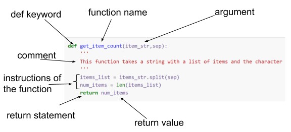
Points to note:

The definition of a function (or procedure) starts with the def keyword and is followed by the name of the function with any parameters used by the function in parentheses.
The definition clause is terminated with a : which causes indentation on the next and subsequent lines. All of these lines form the statements which make up the function. The function ends after the indentation is removed.
Within the function, the parameters behave as variables whose initial values will be those that they were given when the function was called.
functions have a return statement which specifies the value to be returned. This is the value assigned to the variable on the left-hand side of the call to the function. (power in the example above)
You call (run the code) of a function simply by providing its name and values for its parameters the same way you would for any builtin function.
Once the definition of the function has been executed, it becomes part of Python for the current session and can be used anywhere.
Like any other builtin function you can use shift + tab in Jupyter to see the parameters.
At the beginning of the function code we have a multiline comment denoted by the ''' at the beginning and end. This kind of comment is known as a docstring and can be used anywhere in Python code as a documentation aid. It is particularly common, and indeed best practice, to use them to give a brief description of the function at the beginning of a function definition in this way. This is because this description will be displayed along with the parameters when you use the help() function or shift + tab in Jupyter.
The variable x defined within the function only exists within the function, it cannot be used outside in the main program.

In our get_item_count function we have two parameters which must be provided every time the function is used. You need to provide the parameters in the right order or to explicitly name the parameter you are referring to and use the = sign to give it a value.

In many cases of functions we want to provide default values for parameters so the user doesn’t have to. We can do this in the following way

PYTHON

def get_item_count(items_str,sep=';'):
    '''
    This function takes a string with a list of items and the character that they're separated by and returns the number of items
    '''
    items_list = items_str.split(sep)
    num_items = len(items_list)
    return num_items


print(get_item_count(items_owned))

OUTPUT

The only change we have made is to provide a default value for the sep parameter. Now if the user does not provide a value, then the value of 2 will be used. Because items_str is the first parameter we can specify its value by position. We could however have explicitly named the parameters we were referring to.

PYTHON

print(get_item_count(items_owned, sep = ','))
print(get_item_count(items_str = items_owned, sep=';'))

OUTPUT

1
4

Volume of a cube

Write a function definition to calculate the volume of a cuboid. The function will use three parameters h, w and l and return the volume.
Supposing that in addition to the volume I also wanted to calculate the surface area and the sum of all of the edges. Would I (or should I) have three separate functions or could I write a single function to provide all three values together?

Show me the solution

A function to calculate the volume of a cuboid could be:

PYTHON

def calculate_vol_cuboid(h, w, len):
    """
    Calculates the volume of a cuboid.
    Takes in h, w, len, that represent height, width, and length of the cube.
    Returns the volume.
    """
    volume = h * w * len
    return volume

It depends. As a rule-of-thumb, we want our function to do one thing and one thing only, and to do it well. If we always have to calculate these three pieces of information, the ‘one thing’ could be ‘calculate the volume, surface area, and sum of all edges of a cube’. Our function would look like this:

PYTHON

# Method 1 - single function
def calculate_cuboid(h, w, len):
    """
    Calculates information about a cuboid defined by the dimensions h(eight), w(idth), and len(gth).

    Returns the volume, surface area, and sum of edges of the cuboid.
    """
    volume = h * w * len
    surface_area = 2 * (h * w + h * len + len * w)
    edges = 4 * (h + w + len)
    return volume, surface_area, edges

It may be better, however, to break down our function into separate ones - one for each piece of information we are calculating. Our functions would look like this:

PYTHON

# Method 2 - separate functions
def calc_volume_of_cuboid(h, w, len):
    """
    Calculates the volume of a cuboid defined by the dimensions h(eight), w(idth), and len(gth).
    """
    volume = h * w * len
    return volume


def calc_surface_area_of_cuboid(h, w, len):
    """
    Calculates the surface area of a cuboid defined by the dimensions h(eight), w(idth), and len(gth).
    """   
    surface_area = 2 * (h * w + h * len + len * w)
    return surface_area


def calc_sum_of_edges_of_cuboid(h, w, len):
    """
    Calculates the sum of edges of a cuboid defined by the dimensions h(eight), w(idth), and len(gth).
    """   
    sum_of_edges = 4 * (h + w + len)
    return sum_of_edges

We could then rewrite our first solution:

PYTHON

def calculate_cuboid(h, w, len):
    """
    Calculates information about a cuboid defined by the dimensions h(eight), w(idth), and len(gth).

    Returns the volume, surface area, and sum of edges of the cuboid.
    """
    volume = calc_volume_of_cuboid(h, w, len)
    surface_area = calc_surface_area_of_cuboid(h, w, len)
    edges = calc_sum_of_edges_of_cuboid(h, w, len)

    return volume, surface_area, edges

Using libraries

The functions we have created above only exist for the duration of the session in which they have been defined. If you start a new Jupyter notebook you will have to run the code to define them again.

If all of your code is in a single file or notebook this isn’t really a problem.

There are however many (thousands) of useful functions which other people have written and have made available to all Python users by creating libraries (also referred to as packages or modules) of functions.

You can find out what all of these libraries are and their contents by visiting the main (python.org) site.

We need to go through a 2-step process before we can use them in our own programs.

Step 1. use the pip command from the commandline. pip is installed as part of the Python install and is used to fetch the package from the Internet and install it in your Python configuration.

BASH

$ pip install <package name>

pip stands for Python install package and is a commandline function. Because we are using the Anaconda distribution of Python, all of the packages that we will be using in this lesson are already installed for us, so we can move straight on to step 2.

Step 2. In your Python code include an import package-name statement. Once this is done, you can use all of the functions contained within the package.

As all of these packages are produced by 3rd parties independently of each other, there is the strong possibility that there may be clashes in function names. To allow for this, when you are calling a function from a package that you have imported, you do so by prefixing the function name with the package name. This can make for long-winded function names so the import statement allows you to specify an alias for the package name which you must then use instead of the package name.

In future episodes, we will be importing the csv, json, pandas, numpy and matplotlib modules. We will describe their use as we use them.

The code that we will use is shown below

PYTHON

import csv
import json
import pandas as pd
import numpy as np
import matplotlib.pyplot as plt

The first two we don’t alias as they have short names. The last three we do. Matplotlib is a very large library broken up into what can be thought of as sub-libraries. As we will only be using the functions contained in the pyplot sub-library we can specify that explicitly when we import. This saves time and space. It does not effect how we call the functions in our code.

The alias we use (specified after the as keyword) is entirely up to us. However those shown here for pandas, numpy and matplotlib are nearly universally adopted conventions used for these popular libraries. If you are searching for code examples for these libraries on the Internet, using these aliases will appear most of the time.

Key Points

Functions are used to create re-usable sections of code
Using parameters with functions make them more flexible
You can use functions written by others by importing the libraries containing them into your code

Content from Processing data from a file

Last updated on 2023-05-04 | Edit this page

Overview

Questions

How can I read and write files?
What kind of data files can I read?

Objectives

Describe a file handle
Use with open() as to open files for reading and auto-close files
Create and open for writing or appending and auto-close files
Explain what is meant by a record

Reading and Writing datasets

In all of our examples so far, we have directly allocated values to variables in the code we have written before using the variables.

Python has an input() function which will ask for input from the user, but for any large amounts of data this will be an impractical way of collecting data.

The reality is that most of the data that your program uses will be read from a file. Additionally, apart from when you are developing, most of your program output will be written to a file.

In this episode we will look at how to read and write files of data in Python.

There are in fact many different approaches to reading data files and which one you choose will depend on such things as the size of the file and the data format of the file.

In this episode we will;

We will read a file which is in .csv (Comma Separated Values) format.
We will use standard core Python functions to do this
We will read the file one line at a time ( line = record = row of a table)
We will perform simple processing of the file data and print the output
We will split the file into smaller files based on some processing

The file we will be using is only a small file (131 data records), but the approach we are using will work for any size of file. Imagine 131M records. This is because we only process one record at a time so the memory requirements of the programs will be very small. The larger the file the more the processing time required.

Other approaches to reading files will typically expect to read the whole file in one go. This can be efficient when you subsequently process the data but it require large amounts of memory to hold the entire file. We will look at this approach later when the look at the Pandas package.

For our examples in this episode we are going to use the SAFI_results.csv file. This is available for download here and the description of the file is available here.

The code assumes that the file is in the same directory as your notebook.

We will build up our programs in simple steps.

Step 1 - Open the file , read through it and close the file

PYTHON

with open("SAFI_results.csv") as f:       # Open the file and assign it to a new variable which we call 'f'.
                                          # The file will be read-only by default.
                                          # As long as the following code is indented, the file 'f' will be open.
    for line in f:                        # We use a for loop to iterate through the file one line at a time.
        print(line)                       # We simply print the line.
        
print("I'm on to something else now.")    # When we are finished with this file, we stop indenting the code and the file is closed automatically.

OUTPUT

Column1,A01_interview_date,A03_quest_no,A04_start,A05_end,A06_province,A07_district,A08_ward,A09_village,A11_years_farm,A12_agr_assoc,B11_remittance_money,B16_years_liv,B17_parents_liv,B18_sp_parents_liv,B19_grand_liv,B20_sp_grand_liv,B_no_membrs,C01_respondent_roof_type,C02_respondent_wall_type,C02_respondent_wall_type_other,C03_respondent_floor_type,C04_window_type,C05_buildings_in_compound,C06_rooms,C07_other_buildings,D_plots_count,E01_water_use,E17_no_enough_water,E19_period_use,E20_exper_other,E21_other_meth,E23_memb_assoc,E24_resp_assoc,E25_fees_water,E26_affect_conflicts,E_no_group_count,E_yes_group_count,F04_need_money,F05_money_source_other,F06_crops_contr,F08_emply_lab,F09_du_labour,F10_liv_owned_other,F12_poultry,F13_du_look_aftr_cows,F_liv_count,G01_no_meals,_members_count,_note,gps:Accuracy,gps:Altitude,gps:Latitude,gps:Longitude,instanceID

0,17/11/2016,1,2017-03-23T09:49:57.000Z,2017-04-02T17:29:08.000Z,Province1,District1,Ward2,Village2,11,no,no,4,no,yes,no,yes,3,grass,muddaub,,earth,no,1,1,no,2,no,,,,,,,,,2,,,,,no,no,,yes,no,1,2,3,,14,698,-19.11225943,33.48345609,uuid:ec241f2c-0609-46ed-b5e8-fe575f6cefef
...

You can think of the file as being a list of strings. Each string in the list is one complete line from the file.

If you look at the output, you can see that the first record in the file is a header record containing column names. When we read a file in this way, the column headings have no significance, the computer sees them as another record in the file.

Step 2 - Select a specific ‘column’ from the records in the file

We know that the first record in the file is a header record and we want to ignore it. To do this we call the readline() method of the file handle f. We don’t need to assign the line that it will return to a variable as we are not going to use it.

As we read the file the line variable is a string containing a complete record. The fields or columns of the record are separated by each other by “,” as it is a csv file.

As line is a string we can use the split() method to convert it to a list of column values. We are specicically going to select the column which is the 19th entry in the list (remember the list index starts at 0). This refers to the C01_respondent_roof_type column. We are going to examine the different roof types.

PYTHON

with open ("SAFI_results.csv") as f:  # Open the file and assign it to a variable called 'f'.
                                      # Indent the code to keep the file open. Stop indenting to close.
    f.readline()                      # First line is a header so ignore it.

    for line in f:
        print(line.split(",")[18])    # Index 18, the 19th column is C01_respondent_roof_type.

OUTPUT

grass
grass
mabatisloping
mabatisloping
grass
grass
grass
mabatisloping
...

Having a list of the roof types from all of the records is one thing, but it is more likely that we would want a count of each type. By scanning up and down the previous output, there appear to be 3 different types, but we will play safe and assume there may be more.

Step 3 - How many of each different roof types are there?

PYTHON

# 1
with open ("SAFI_results.csv") as f:

# 2
    f.readline()

# 3
    grass_roof = 0
    mabatisloping_roof = 0
    mabatipitched_roof = 0
    roof_type_other = 0

    for line in f:
# 4
        roof_type = line.split(",")[18]
# 5    
        if roof_type == 'grass' :
            grass_roof += 1
        elif roof_type == 'mabatisloping' :
            mabatisloping_roof += 1
        elif roof_type == 'mabatipitched' :
            mabatipitched_roof += 1
        else :
            roof_type_other += 1

#6
print("There are ", grass_roof, " grass roofs")
print("There are ", mabatisloping_roof, " mabatisloping roofs")
print("There are ", mabatipitched_roof, " mabatipitchedg roofs")
print("There are ", roof_type_other, " other roof types")

OUTPUT

There are 73 grass roofs
There are 48 mabatisloping roofs
There are 10 mabatipitchedg roofs
There are 0 other roof types

What are we doing here?

Open the file
Ignore the headerline
Initialise roof type variables to 0
Extract the C01_respondent_roof_type information from each record
Increment the appropriate variable
Print out the results (we have stopped indenting so the file will be closed)

Instead of printing out the counts of the roof types, you may want to extract all of one particular roof type to a separate file. Let us assume we want all of the grass roof records to be written to a file.

PYTHON

# 1
with open ("SAFI_results.csv") as fr:              # Note how we have used a new variable name, 'fr'.
                                                   # The file is read-only by default.

    with open ("SAFI_grass_roof.csv", "w") as fw:  # We are keeping 'fr' open so we indent.
                                                   # We specify a second parameter, "w" to make this file writeable.
                                                   # We use a different variable, 'fw'.
        for line in fr:
# 2    
            if line.split(",")[18] == 'grass' :
                fw.write(line)

What are we doing here?

Open the files. Because there are now two files, each has its own file handle: fr for the file we read and fw for the file we are going to write. (They are just variable names so you can use anything you like). For the file we are going to write to we use w for the second parameter. If the file does not exist it will be created. If it does exist, then the contents will be overwritten. If we want to append to an existing file we can use a as the second parameter.
Because we are just testing a specific field from the record to have a certain value, we don’t need to put it into a variable first. If the expression is True, then we use write() method to write the complete line just as we read it to the output file.

In this example we didn’t bother skipping the header line as it would fail the test in the if statement. If we did want to include it we could have added the line

PYTHON

fw.write(fr.readline())

before the for loop

Exercise

From the SAFI_results.csv file extract all of the records where the C01_respondent_roof_type (index 18) has a value of 'grass' and the C02_respondent_wall_type (index 19) has a value of 'muddaub' and write them to a file. Within the same program write all of the records where C01_respondent_roof_type (index 18) has a value of 'grass' and the C02_respondent_wall_type (index 19) has a value of 'burntbricks' and write them to a separate file. In both files include the header record.

Show me the solution

PYTHON

with open ("SAFI_results.csv") as fr:

   with open ("SAFI_grass_roof_muddaub.csv", "w") as fw1:
      with open ("SAFI_grass_roof_burntbricks.csv", "w") as fw2:

          headerline = fr.readline()
          fw1.write(headerline)
          fw2.write(headerline)

          for line in fr:
              if line.split(",")[18] == 'grass' :
                  if line.split(",")[19] == 'muddaub' :
                      fw1.write(line)
                  if line.split(",")[19] == 'burntbricks' :
                      fw2.write(line)

In our example of printing the counts for the roof types, we assumed that we knew what the likely roof types were. Although we did have an 'other' option to catch anything we missed. Had there been any we would still be non the wiser as to what they represented. We were able to decide on the specific roof types by manually scanning the list of C01_respondent_roof_type values. This was only practical because of the small file size. For a multi-million record file we could not have done this.

We would like a way of creating a list of the different roof types and at the same time counting them. We can do this by using not a Python list structure, but a Python dictionary.

The Python dictionary structure

In Python a dictionary object maps keys to values. A dictionary can hold any number of keys and values but a key cannot be duplicated.

The following code shows examples of creating a dictionary object and manipulating keys and values.

PYTHON

# an empty dictionary
myDict = {}

# A dictionary with a single Key-value pair

personDict = {'Name' : 'Peter'}

# I can add more about 'Peter' to the dictionary

personDict['Location'] = 'Manchester'


# I can print all of the keys and values from the dictionary

print(personDict.items())

# I can print all of the keys and values from the dictionary - and make it look a bit nicer

for item in personDict:
    print(item, "=", personDict[item])

# or all of the keys

print(personDict.keys())

# or all of the values

print(personDict.values())

# I can access the value for a given key

x = personDict['Name']
print(x)

# I can change value for a given key

personDict['Name'] = "Fred"
print(personDict['Name'])

# I can check if a key exists

key = 'Name'

if key in personDict :
    print("already exists")
else :
    personDict[key] = "New value"

OUTPUT

dict_items([('Location', 'Manchester'), ('Name', 'Peter')])
Location = Manchester
Name = Peter
dict_keys(['Location', 'Name'])
dict_values(['Manchester', 'Peter'])
Peter
Fred
already exists

Exercise

Create a dictionary called dict_roof_types with initial keys of type1 and type2 and give them values of 1 and 3.
Add a third key type3 with a value of 6.
Add code to check if a key of type4 exists. If it does not add it to the dictionary with a value of 1 if it does, increment its value by 1
Add code to check if a key of type2 exists. If it does not add it to the dictionary with a value of 1 if it does, increment its value by 1
Print out all of the keys and values from the dictionary

Show me the solution

PYTHON


# 1
dict_roof_types = {'type1' : 1 , 'type2' : 3}

# 2
dict_roof_types['type3'] = 6

# 3
key = 'type4'
if key in dict_roof_types :
    dict_roof_types[key] += 1
else :
    dict_roof_types[key] = 1

# 4
key = 'type2'
if key in dict_roof_types :
    dict_roof_types[key] += 1
else :
    dict_roof_types[key] = 1
 
# 5
for item in dict_roof_types:
    print(item, "=", dict_roof_types[item])

We are now in a position to re-write our count of roof types example without knowing in advance what any of the roof types are.

PYTHON

# 1
with open ("SAFI_results.csv") as f:

# 2
    f.readline()

# 3
    dict_roof_types = {}

    for line in f:
# 4
        roof_type = line.split(",")[18]
# 5    
        if roof_type in dict_roof_types :
            dict_roof_types[roof_type] += 1
        else :
            dict_roof_types[roof_type] = 1

# 6

for item in dict_roof_types:
    print(item, "=", dict_roof_types[item])

OUTPUT

grass = 73
mabatisloping = 48
mabatipitched = 10

What are we doing here?

Open the file
Ignore the headerline
Create an empty dictionary
Extract the C01_respondent_roof_type information from each record
Either add to the dictionary with a value of 1 or increment the current value for the key by 1
Print out the contents of the dictionary (stopped indenting so file is closed)

You can apply the same approach to count values in any of the fields/columns of the file.

Key Points

Reading data from files is far more common than program ‘input’ requests or hard coding values
Python provides simple means of reading from a text file and writing to a text file
Tabular data is commonly recorded in a ‘csv’ file
Text files like csv files can be thought of as being a list of strings. Each string is a complete record
You can read and write a file one record at a time
Python has builtin functions to parse (split up) records into individual tokens

Content from Dates and Time

Last updated on 2023-05-04 | Edit this page

Overview

Questions

How are dates and time represented in Python?
How can I manipulate dates and times?

Objectives

Describe some of the datetime functions available in Python
Describe the use of format strings to describe the layout of a date and/or time string
Make use of date arithmetic

Date and Times in Python

Python can be very flexible in how it interprets ‘strings’ which you want to be considered as a date, time, or date and time, but you have to tell Python how the various parts of the date and/or time are represented in your ‘string’. You can do this by creating a format. In a format, different case sensitive characters preceded by the % character act as placeholders for parts of the date/time, for example %Y represents year formatted as 4 digit number such as 2014.

A full list of the characters used and what they represent can be found towards the end of the datetime section of the official Python documentation.

There is a today() method which allows you to get the current date and time. By default it is displayed in a format similar to the ISO 8601 standard format.

To use the date and time functions you need to import the datetime module.

PYTHON

from datetime import datetime

today = datetime.today()
print('ISO     :', today)

OUTPUT

ISO     : 2018-04-12 16:19:17.177441

We can use our own formatting instead. For example, if we wanted words instead of number and the 4 digit year at the end we could use the following.

PYTHON

format = "%a %b %d %H:%M:%S %Y"

today_str = today.strftime(format)
print('strftime:', today_str)
print(type(today_str))

today_date = datetime.strptime(today_str, format)
print('strptime:', today_date.strftime(format))
print(type(today_date))

OUTPUT

strftime: Thu Apr 12 16:19:17 2018
<class 'str'>
strptime: Thu Apr 12 16:19:17 2018
<class 'datetime.datetime'>

strftime converts a datetime object to a string and strptime creates a datetime object from a string. When you print them using the same format string, they look the same.

The format of the date fields in the SAFI_results.csv file have been generated automatically to comform to the ISO 8601 standard.

When we read the file and extract the date fields, they are of type string. Before we can use them as dates, we need to convert them into Python date objects.

In the format string we use below, the - , : , T and Z characters are just that, characters in the string representing the date/time. Only the character preceded with % have special meanings.

Having converted the strings to datetime objects, there are a variety of methods that we can use to extract different components of the date/time.

PYTHON

from datetime import datetime


format = "%Y-%m-%dT%H:%M:%S.%fZ"
f = open('SAFI_results.csv', 'r')

#skip the header line
line = f.readline()

# next line has data
line = f.readline()

strdate_start = line.split(',')[3]  # A04_start
strdate_end = line.split(',')[4]    # A05_end

print(type(strdate_start), strdate_start)
print(type(strdate_end), strdate_end)


# the full date and time
datetime_start = datetime.strptime(strdate_start, format)
print(type(datetime_start))
datetime_end = datetime.strptime(strdate_end, format)

print('formatted date and time', datetime_start)
print('formatted date and time', datetime_end)


# the date component
date_start = datetime.strptime(strdate_start, format).date()
print(type(date_start))
date_end = datetime.strptime(strdate_end, format).date()

print('formatted start date', date_start)
print('formatted end date', date_end)

# the time component
time_start = datetime.strptime(strdate_start, format).time()
print(type(time_start))
time_end = datetime.strptime(strdate_end, format).time()

print('formatted start time', time_start)
print('formatted end time', time_end)


f.close()

OUTPUT

<class 'str'> 2017-03-23T09:49:57.000Z
<class 'str'> 2017-04-02T17:29:08.000Z
<class 'datetime.datetime'>
formatted date and time 2017-03-23 09:49:57
formatted date and time 2017-04-02 17:29:08
<class 'datetime.date'>
formatted start date 2017-03-23
formatted end date 2017-04-02
<class 'datetime.time'>
formatted start time 09:49:57
formatted end time 17:29:08

Components of dates and times

For a date or time we can also extract individual components of them. They are held internally in the datetime datastructure.

PYTHON

# date parts.
print('formatted end date', date_end)
print(' end date year', date_end.year)
print(' end date month', date_end.month)
print(' end date day', date_end.day)
print (type(date_end.day))

# time parts.

print('formatted end time', time_end)
print(' end time hour', time_end.hour)
print(' end time minutes', time_end.minute)
print(' end time seconds', time_end.second)
print(type(time_end.second))

OUTPUT

formatted end date 2017-04-02
 end date year 2017
 end date month 4
 end date day 2
<class 'int'>
formatted end time 17:29:08
 end time hour 17
 end time minutes 29
 end time seconds 8
<class 'int'>

Date arithmetic

We can also do arithmetic with the dates.

PYTHON

date_diff = datetime_end - datetime_start
date_diff
print(type(datetime_start))
print(type(date_diff))
print(date_diff)

date_diff = datetime_start - datetime_end
print(type(date_diff))
print(date_diff)

OUTPUT

<class 'datetime.datetime'>
<class 'datetime.timedelta'>
10 days, 7:39:11
<class 'datetime.timedelta'>
-11 days, 16:20:49

Exercise

How do you interpret the last result?

The code below calculates the time difference between supposedly starting the survey and ending the survey (for each respondent).

PYTHON

from datetime import datetime

format = "%Y-%m-%dT%H:%M:%S.%fZ"

f = open('SAFI_results.csv', 'r')

line = f.readline()

for line in f:
    #print(line)
    strdate_start = line.split(',')[3]
    strdate_end = line.split(',')[4]

    datetime_start = datetime.strptime(strdate_start, format)
    datetime_end = datetime.strptime(strdate_end, format)
    date_diff = datetime_end - datetime_start
    print(datetime_start, datetime_end, date_diff )


f.close()

OUTPUT

2017-03-23 09:49:57 2017-04-02 17:29:08 10 days, 7:39:11
2017-04-02 09:48:16 2017-04-02 17:26:19 7:38:03
2017-04-02 14:35:26 2017-04-02 17:26:53 2:51:27
2017-04-02 14:55:18 2017-04-02 17:27:16 2:31:58
2017-04-02 15:10:35 2017-04-02 17:27:35 2:17:00
2017-04-02 15:27:25 2017-04-02 17:28:02 2:00:37
2017-04-02 15:38:01 2017-04-02 17:28:19 1:50:18
2017-04-02 15:59:52 2017-04-02 17:28:39 1:28:47
2017-04-02 16:23:36 2017-04-02 16:42:08 0:18:32
...

Exercise

In the SAFI_results.csv file the A01_interview_date field (index 1) contains a date in the form of ‘dd/mm/yyyy’. Read the file and calculate the differences in days (because the interview date is only given to the day) between the A01_interview_date values and the A04_start values. You will need to create a format string for the A01_interview_date field.
Looking at the results here and from the previous section of code. Do you think the use of the smartphone data entry system for the survey was being used in real time?

Show me the solution

PYTHON

from datetime import datetime

format1 = "%Y-%m-%dT%H:%M:%S.%fZ"
format2 = "%d/%m/%Y"

f = open('SAFI_results.csv', 'r')

line = f.readline()

for line in f:
    A01 = line.split(',')[1]
    A04 = line.split(',')[3]
   
    datetime_A04 = datetime.strptime(A04, format1)
    datetime_A01 = datetime.strptime(A01, format2)
    date_diff = datetime_A04 - datetime_A01
    print(datetime_A04, datetime_A01, date_diff.days )
     
f.close()

Key Points

Date and Time functions in Python come from the datetime library, which needs to be imported
You can use format strings to have dates/times displayed in any representation you like
Internally date and times are stored in special data structures which allow you to access the component parts of dates and times

Content from Processing JSON data

Last updated on 2023-05-04 | Edit this page

Overview

Questions

What is JSON format?
How can I extract specific data items from a JSON record?
How can I convert an array of JSON record into a table?

Objectives

Describe the JSON data format
Understand where JSON is typically used
Appreciate some advantages of using JSON over tabular data
Appreciate some dis-advantages of processing JSON documents
Compare JSON to the Python Dict data type
Use the JSON package to read a JSON file
Display formatted JSON
Select and display specific fields from a JSON document
Write tabular data from selected elements from a JSON document to a csv file

More on Dictionaries

In the Processing data from file episode we introduced the dictionary object.

We created dictionaries and we added key : value pairs to the dictionary.

In all of the examples that we used, the value was always a simple data type like an integer or a string.

The value associated with a key in a dictionary can be of any type including a list or even another dictionary.

We created a simple dictionary object with the following code:

PYTHON

personDict = {'Name' : 'Peter'}
personDict['Location'] = 'Manchester'

print(personDict)

OUTPUT

{'Name': 'Peter', 'Location': 'Manchester'}

So far the keys in the dictionary each relate to a single piece of information about the person. What if we wanted to add a list of items?

PYTHON

personDict['Children'] = ['John', 'Jane', 'Jack']
personDict['Children_count'] = 3
print(personDict)

OUTPUT

{'Name': 'Peter', 'Children': ['John', 'Jane', 'Jack'], 'Children_count': 3, 'Location': 'Manchester'}

Not only can I have a key where the value is a list, the value could also be another dictionary object. Suppose I want to add some telephone numbers

PYTHON

personDict['phones'] = {'home' : '0102345678', 'mobile' : '07770123456'}
print(personDict.values())

# adding another phone
personDict['phones']['business'] =  '0161234234546'
print(personDict)

OUTPUT

dict_values(['Peter', ['John', 'Jane', 'Jack'], {'home': '0102345678', 'mobile': '07770123456'}, 3, 'Manchester'])
{'Name': 'Peter', 'Children': ['John', 'Jane', 'Jack'], 'phones': {'home': '0102345678', 'mobile': '07770123456', 'business': '0161234234546'}, 'Children_count': 3, 'Location': 'Manchester'}

Exercise

Using the personDict as a base add information relating to the persons home and work addresses including postcodes.
Print out the postcode for the work address.
Print out the names of the children on seperate lines (i.e. not as a list)

Show me the solution

PYTHON

personDict['Addresses'] = {'Home' : {'Addressline1' : '23 acacia ave.', 'Addressline2' : 'Romford', 'PostCode' : 'RO6 5WR'},
                          'Work' : {'Addressline1' : '19 Orford Road.', 'Addressline2' : 'London', 'PostCode' : 'EC4J 3XY'}
                          }

print(personDict['Addresses']['Work']['PostCode'])

for child in personDict['Children']:
    print(child)

The ability to create dictionaries containing lists and other dictionaries, makes the dictionary object very versatile, you can create an arbitrarily complex data structure of dictionaries within dictionaries.

In practice you will not be doing this manually, instead like most data you will read it in from a file.

The JSON data format

The JSON data format was designed as a way of allowing different machines or processes within machines to communicate with each other by sending messages constructed in a well defined format. JSON is now the preferred data format used by APIs (Application Programming Interfaces).

The JSON format although somewhat verbose is not only Human readable but it can also be mapped very easily to a Python dictionary object.

We are going to read a file of data formatted as JSON, convert it into a dictionary object in Python then selectively extract Key-Value pairs and create a csv file from the extracted data.

The JSON file we are going to use is the SAFI.json file. This is the output file from an electronic survey system called ODK. The JSON represents the answers to a series of survey questions. The questions themselves have been replaced with unique Keys, the values are the answers.

Because detailed surveys are by nature nested structures making it possible to record different levels of detail or selectively ask a set of specific questions based on the answer given a previous question, the structure of the answers for the survey can not only be complex and convoluted, it could easily be different from one survey respondent’s set of answers to another.

Advantages of JSON

Very popular data format for APIs (e.g. results from an Internet search)
Human readable
Each record (or document as they are called) is self contained. The equivalent of the column name and column values are in every record.
Documents do not all have to have the same structure within the same file
Document structures can be complex and nested

Dis-advantages of JSON

It is more verbose than the equivalent data in csv format
Can be more difficult to process and display than csv formatted data

Viewing JSON data

JSON can often be viewed directly in the web browsers: example.
Browser extensions are often available for ease of viewing JSON data e.g., Chrome, Firefox, Safari, etc.
JSON files can be opened using text editors e.g., notepad, nano, textedit, etc.
There are many websites which allow viewing or beautifying JSON data with ease. For example, http://jsonviewer.stack.hu/. Try pasting or loading JSON data in the second tab called “text” on that website and then clicking on the “format” button. Clicking on the first tab, “viewer” also gives another view of the data.

Use the JSON package to read a JSON file

PYTHON

import json

with open('SAFI.json') as json_data:
    d = json.load(json_data)
    print(type(d))
    print(type(d[0]))
    print(json.dumps(d[0], indent=2))

OUTPUT

<class 'list'>
<class 'dict'>
{
  "G02_months_lack_food": [
    "Jan"
  ],
  "G01_no_meals": 2,
  "E_no_group_count": "2",
  "A03_quest_no": "01",
...

Points to note:

We import the json package with an import statement.
We have chosen to use the with statement to open the SAFI.json file. Notice the : at the end of the line and the subsequent indentation. The with statement is in effect until we un-indent. At which time the file will automatically be closed. So we don’t need to do so explicitly.
‘json_data’ is the file handle.
The json.load method is passed the file handle and reads the complete file.
The variable d is a list of dictionaries. (When we read the csv file we considered it to be a list of strings).
The json.dumps method can be used to print either the entire file or a specific dictionary from the list in a formatted manner by using the indent parameter)

By default the order in which the keys of the dictionary are printed is not guaranteed. If we want them in sorted order we can have them sorted by using the sort_keys parameter

PYTHON

print(json.dumps(d[0], indent=2, sort_keys=True))

OUTPUT

{
  "A01_interview_date": "2016-11-17",
  "A03_quest_no": "01",
  "A04_start": "2017-03-23T09:49:57.000Z",
  "A05_end": "2017-04-02T17:29:08.000Z",
  "A06_province": "province1",
...
}

Extracting specific fields from a JSON document

If we want to extract fields from a JSON document, the first step isto convert the JSON document into a Python dictionary. We have in fact already done this with the

PYTHON

d = json.load(json_data)

line. d a list object and each entry in the list is a Dictionary object.

Extract the fields we want into a flat format

Despite the arbitrary complexity of a JSON document or a Python dictionary object, we can adopt a very systematic approach to extracting individual fields form the structure.

The story so far: Our JSON file has been read into a variable d. We know that d is a list of dictionaries. Each dictionary represents a JSON document ( a record).

We can print the contents of the first dictionary in the list with

PYTHON

print(json.dumps(d[0], indent=2, sort_keys=True))

Exercise

In the output from the code above there is a key with the name of D_curr_crop. Find it and by looking at the indentation and the [ (lists) and { (dictionaries) describe in English how you could find the first occurrence of D_curr_crop starting with d.
Use a print statement to find out what it is.

Show me the solution

d is a list of dictionaries
d[0] is the first dictionary
within d[0] there is a key D_plots whose value is a list and contains dictionaries
d[0]['D_plots'][0] is the first dictionary in the list
within d[0]['D_plots'][0] there is a key D_crops which is also a list of dictionaries
d[0]['D_plots'][0]['D_crops'][0] is the first dictionary in the list
within this dictionary there is a key D_curr_crop

Being able to start at the outermost level and work your way in is very important when you need to extract specific items.

PYTHON

print(d[0]['D_plots'][0]['D_crops'][0]['D_curr_crop'])

Being able to drill down in this way is very useful in helping you get a feel for the JSON data structure. In practice it is more likely that instead of returning the first occurrence of D_curr_crop you will want to return all of them. This requires a little more programming and to be aware of two potential problems.

D_curr_crop may not exist in any particular dictionary within D_crops
any of the lists D_plots or D_crops could be missing or just empty lists ([])

In our first attempt we will ignore these problems.

PYTHON

for farms in d:
    plot = farms['D_plots']
    for crops in plot:
        crop = crops['D_crops']
        for curr_crops in crop:
            print(curr_crops['D_curr_crop'])

OUTPUT

maize
maize
maize
tomatoes
vegetable
maize
maize
maize
sorghum
...

In this version we test if all of the keys exist. This could be extended to check that the lists are not empty.

PYTHON

for farms in d:
    if 'D_plots' in farms :
        plot = farms['D_plots']
        for crops in plot:
            if 'D_crops' in crops :
                crop = crops['D_crops']
                for curr_crops in crop:
                    if 'D_curr_crop' in curr_crops:
                        print(curr_crops['D_curr_crop'])

We can now produce a list of all of the crops in all of the plots in all of the farms.

We can also create a unique set of all of the crops grown using the Python set data structure as shown in the code below. A set is like a list but does not allow duplicate values (but doesn’t raise an error if you try to add a duplicate).

PYTHON

unique_crops = set()
for farms in d:
    if 'D_plots' in farms :
        plot = farms['D_plots']
        for crops in plot:
            if 'D_crops' in crops :
                crop = crops['D_crops']
                for curr_crops in crop:
                    if 'D_curr_crop' in curr_crops:
                        #print(curr_crops['D_curr_crop'])
                        unique_crops.add(curr_crops['D_curr_crop'])
print(unique_crops)

OUTPUT

{'peanut', 'potatoes', 'tomatoes', 'other', 'vegetable', 'amendoim', 'sunflower', 'bananas', 'sesame', None, 'cucumber', 'onion', 'sorghum', 'piri_piri', 'baby_corn', 'cabbage', 'ngogwe', 'maize', 'pigeonpeas', 'beans'}

Simply having a list of all of the crops is unlikely to be enough. What you are really interested in is which farm grows which crops in which plot.

We can accumulate this information as we move through the list of dictionary objects. At the top level, farm, there is a unique identifier A03_quest_no which we can use. for the plot and the crop within the plot we will create our own simple indexing system (plot_no and crop_no). At the end instead of just printing the crop name, we also print the details of where this crop is being grown.

PYTHON

for farms in d:
    plot_no = 0
    id = farms['A03_quest_no']
    if 'D_plots' in farms :
        plot = farms['D_plots']
        for crops in plot:
            crop_no = 0
            plot_no += 1
            if 'D_crops' in crops :
                crop = crops['D_crops']
                for curr_crops in crop:
                    crop_no += 1
                    if 'D_curr_crop' in curr_crops:
                        print("Farm no ", id," grows ", curr_crops['D_curr_crop']," in plot", plot_no , " and it is crop number ", crop_no)

OUTPUT

Farm no 01 grows maize in plot 1 and it is crop number 1
Farm no 01 grows maize in plot 2 and it is crop number 1
Farm no 01 grows maize in plot 1 and it is crop number 1
Farm no 01 grows tomatoes in plot 2 and it is crop number 1
Farm no 01 grows vegetable in plot 3 and it is crop number 1
...

The final stage of this data extraction process is to save the extracted data to a file for subsequent use.

Rather than manually appending all of the information items into a string with , seperating each, we can use the csv module.

To do this we need to create a csv.writer object and use it to write complete rows of data at a time. csv.writer expects the data to be provided as a list of items.

For the header row we provide a list of strings containing the colmn names we want and at the end we proivide the data items in a list as well.

PYTHON

import csv
filename = "SAFI_crops.csv"
fw = open(filename, 'w')
cf = csv.writer(fw, lineterminator='\n')

# write the header
cf.writerow(["Farm","plot_no","plot_area","crop_no","crop_name"])

for farms in d:
    plot_no = 0
    id = farms['A03_quest_no']
    if 'D_plots' in farms :
        plot = farms['D_plots']
        for crops in plot:
            crop_no = 0
            plot_no += 1
            if 'D_crops' in crops :
                plot_area = crops['D02_total_plot']
                crop = crops['D_crops']
                for curr_crops in crop:
                    crop_no += 1
                    if 'D_curr_crop' in curr_crops:
                        #print( id, plot_no , plot_area , crop_no, curr_crops['D_curr_crop'])
                        cf.writerow([id, plot_no , plot_area , crop_no, curr_crops['D_curr_crop']])

fw.close()

Key Points

JSON is a popular data format for transferring data used by a great many Web based APIs
The JSON data format is very similar to the Python Dictionary structure.
The complex structure of a JSON document means that it cannot easily be ‘flattened’ into tabular data
We can use Python code to extract values of interest and place them in a csv file

Content from Reading data from a file using Pandas

Last updated on 2023-05-04 | Edit this page

Overview

Questions

What is Pandas?
How do I read files using Pandas?
What is the difference between reading files using Pandas and other methods of reading files?

Objectives

Explain what a module is and how they are used in Python
Describe what the Python Data Analysis Library (pandas) is
Load the Python Data Analysis Library (pandas)
Use read_csv to read tabular data into Python

What is Pandas?

pandas is a Python library containing a set of functions and specialised data structures that have been designed to help Python programmers to perform data analysis tasks in a structured way.

Most of the things that pandas can do can be done with basic Python, but the collected set of pandas functions and data structure makes the data analysis tasks more consistent in terms of syntax and therefore aids readabilty.

Particular features of pandas that we will be looking at over this and the next couple of episodes include:

Reading data stored in CSV files (other file formats can be read as well)
Slicing and subsetting data in Dataframes (tables!)
Dealing with missing data
Reshaping data (long -> wide, wide -> long)
Inserting and deleting columns from data structures
Aggregating data using data grouping facilities using the split-apply-combine paradigm
Joining of datasets (after they have been loaded into Dataframes)

If you are wondering why I write pandas with a lower case ‘p’ it is because it is the name of the package and Python is case sensitive.

Importing the pandas library

Importing the pandas library is done in exactly the same way as for any other library. In almost all examples of Python code using the pandas library, it will have been imported and given an alias of pd. We will follow the same convention.

PYTHON

import pandas as pd

Pandas data structures

There are two main data structure used by pandas, they are the Series and the Dataframe. The Series equates in general to a vector or a list. The Dataframe is equivalent to a table. Each column in a pandas Dataframe is a pandas Series data structure.

We will mainly be looking at the Dataframe.

We can easily create a Pandas Dataframe by reading a .csv file

Reading a csv file

When we read a csv dataset in base Python we did so by opening the dataset, reading and processing a record at a time and then closing the dataset after we had read the last record. Reading datasets in this way is slow and places all of the responsibility for extracting individual data items of information from the records on the programmer.

The main advantage of this approach, however, is that you only have to store one dataset record in memory at a time. This means that if you have the time, you can process datasets of any size.

In Pandas, csv files are read as complete datasets. You do not have to explicitly open and close the dataset. All of the dataset records are assembled into a Dataframe. If your dataset has column headers in the first record then these can be used as the Dataframe column names. You can explicitly state this in the parameters to the call, but pandas is usually able to infer that there ia a header row and use it automatically.

For our examples in this episode we are going to use the SN7577.tab file. This is available for download here and the description of the file is available here

We are going to read in our SN7577.tab file. Although this is a tab delimited file we will still use the pandas read_csv method, but we will explicitly tell the method that the separator is the tab character and not a comma which is the default.

PYTHON

df_SN7577 = pd.read_csv("SN7577.tab", sep='\t')

Exercise

What happens if you forget to specify sep='\t' when reading a tab delimited dataset

Show me the solution

PYTHON

df_SN7577_oops = pd.read_csv("SN7577.tab")
print(df_SN7577_oops.shape)
print(df_SN7577_oops)

If you allow pandas to assume that your columns are separated by commas (the default) and there aren’t any, then each record will be treated as a single column. So the shape is given as 1286 rows (correct) but only one column. When the contents is display the only column name is the complete first record. Notice the \t used to represent the tab characters in the output. This is the same format we used to specify the tab separator when we correctly read in the file.

Getting information about a Dataframe

You can find out the type of the variable df_SN7577 by using the type function.

PYTHON

print(type(df_SN7577))

OUTPUT

<class 'pandas.core.frame.DataFrame'>

You can see the contents by simply entering the variable name. You can see from the output that it is a tabular format. The column names have been taken from the first record of the file. On the left hand side is a column with no name. The entries here have been provided by pandas and act as an index to reference the individual rows of the Dataframe.

The read_csv() function has an index_col parameter which you can use to indicate which of the columns in the file you wish to use as the index instead. As the SN7577 dataset doesn’t have a column which would uniquely identify each row we cannot do that.

Another thing to notice about the display is that it is truncated. By default you will see the first and last 30 rows. For the columns you will always get the first few columns and typically the last few depending on display space.

PYTHON

df_SN7577

Similar information can be obtained with df_SN7577.head() But here you are only returned the first 5 rows by default.

PYTHON

df_SN7577.head()

Exercise

As well as the head() method there is a tail() method. What do you think it does? Try it.
Both methods accept a single numeric parameter. What do you think it does? Try it.

You can obtain other basic information about your Dataframe of data with:

PYTHON

# How many rows?
print(len(df_SN7577))
# How many rows and columns - returned as a tuple
print(df_SN7577.shape)
#How many 'cells' in the table
print(df_SN7577.size)
# What are the column names
print(df_SN7577.columns)
# what are the data types of the columns?
print(df_SN7577.dtypes)

OUTPUT

1286
(1286, 202)
259772
Index(['Q1', 'Q2', 'Q3', 'Q4', 'Q5ai', 'Q5aii', 'Q5aiii', 'Q5aiv', 'Q5av',
       'Q5avi',
       ...
       'numhhd', 'numkid', 'numkid2', 'numkid31', 'numkid32', 'numkid33',
       'numkid34', 'numkid35', 'numkid36', 'wts'],
      dtype='object', length=202)
Q1             int64
Q2             int64
Q3             int64
...
Length: 202, dtype: object

Exercise

When we asked for the column names and their data types, the output was abridged, i.e. we didn’t get the values for all of the columns. Can you write a small piece of code which will return all of the values

Show me the solution

PYTHON

for name in df_SN7577.columns:
    print(name)

Key Points

pandas is a Python library containing functions and data structures to assist in data analysis
pandas data structures are the Series (like a vector) and the Dataframe (like a table)
the pandas read_csv function allows you to read an entire csv file into a Dataframe

Content from Extracting row and columns

Last updated on 2023-05-04 | Edit this page

Overview

Questions

How can I extract specific rows and columns from a Dataframe?
How can I add or delete columns from a Dataframe?
How can I find and change missing values in a Dataframe?

Objectives

Define indexing as it relates to data structures
Select specific columns from a data frame
Select specific rows from a data frame based on conditional expressions
Using indexes to access rows and columns
Copy a data frame
Add columns to a data frame
Analyse datasets having missing/null values

We will continue this episode from where we left off in the last episode. If you have restarted Jupyter or you want to use a new notebook make sure that you import pandas and have read the SN7577.tab dataset into a Dataframe.

PYTHON

import pandas as pd
df_SN7577 = pd.read_csv("SN7577.tab", sep='\t')

Selecting rows and columns from a pandas Dataframe

If we know which columns we want before we read the data from the file we can tell read_csv() to only import those columns by specifying columns either by their index number (starting at 0) as a list to the usecols parameter. Alternatively we can also provide a list of column names.

PYTHON

df_SN7577_some_cols = pd.read_csv("SN7577.tab", sep='\t', usecols= [0,1,2,173,174,175])
print(df_SN7577_some_cols.shape)
print(df_SN7577_some_cols.columns)
df_SN7577_some_cols = pd.read_csv("SN7577.tab", sep='\t', usecols= ['Q1', 'Q2', 'Q3', 'sex', 'age', 'agegroups'])
print(df_SN7577_some_cols.columns)

OUTPUT

(1286, 6)
Index(['Q1', 'Q2', 'Q3', 'sex', 'age', 'agegroups'], dtype='object')
Index(['Q1', 'Q2', 'Q3', 'sex', 'age', 'agegroups'], dtype='object')

Let us assume for now that we read in the complete file which is now in the Dataframe df_SN7577, how can we now refer to specific columns?

There are two ways of doing this using the column names (or labels):

PYTHON

# Both of these statements are the same
print(df_SN7577['Q1'])
# and
print(df_SN7577.Q1)

OUTPUT

If we are interested in more than one column, the 2nd method above cannot be used. However in the first, although we used a string with the value of 'Q1' we could also have provided a list of strings. Remember that lists are enclosed in [].

PYTHON

print(df_SN7577[['Q1', 'Q2', 'Q3']])

PYTHON

Q1  Q2  Q3
0      1  -1   1
1      3  -1   1
2     10   3   2
3      9  -1  10
...

Exercise

What happens if you:

List the columns you want out of order from the way they appear in the file?
Put the same column name in twice?
Put in a non-existing column name? (a.k.a Typo)

Show me the solution

PYTHON

print(df_SN7577[['Q3', 'Q2']])
print(df_SN7577[['Q3', 'Q2', 'Q3']])
print(df_SN7577[['Q33', 'Q2']])

Filtering by Rows

You can filter the Dataframe by rows by specifying a range in the form of a:b. a is the first row and b is one beyond the last row required.

PYTHON

# select row with index of 1, 2 and 3 (rows 2, 3 and 4 in the Dataframe)
df_SN7577_some_rows = df_SN7577[1:4]
df_SN7577_some_rows

Exercise

What happens if we ask for a single row instead of a range?

Show me the solution

PYTHON

df_SN7577[1]

You get an error if you only specify 1. You need to use :1 or 0:1 to get the first row returned. The : is always required. You can use : by itself to return all of the rows.

Using criteria to filter rows

It is more likely that you will want to select rows from the Dataframe based on some criteria, such as “all rows where the value for Q2 is -1”.

PYTHON

df_SN7577_some_rows = df_SN7577[(df_SN7577.Q2 == -1)]
df_SN7577_some_rows

The criteria can be more complex and isn’t limited to a single column’s values:

PYTHON

df_SN7577_some_rows = df_SN7577[ (df_SN7577.Q2 == -1) & (df_SN7577.numage > 60)]
df_SN7577_some_rows

We can combine the row selection with column selection:

PYTHON

df_SN7577_some_rows = df_SN7577[ (df_SN7577.Q2 == -1) & (df_SN7577.numage > 60)][['Q1', 'Q2','numage']]
df_SN7577_some_rows

Selecting rows on the row index is of limited use unless you need to select a contiguous range of rows.

There is however another way of selecting rows using the row index:

PYTHON

df_SN7577_some_rows = df_SN7577.iloc[1:4]
df_SN7577_some_rows

Using the iloc method gives the same results as our previous example.

However, now we can specify a single value and more importantly we can use the range() function to indicate the records that we want. This can be useful for making pseudo-random selections of rows from across the Dataframe.

PYTHON

# Select the first row from the Dataframe
df_SN7577_some_rows = df_SN7577.iloc[0]
df_SN7577_some_rows
# select every 100th record from the Dataframe.
df_SN7577_some_rows = df_SN7577.iloc[range(0, len(df_SN7577), 100)]
df_SN7577_some_rows

You can also specify column ranges using the iloc method again using the column index numbers:

PYTHON

# columns 0,1,2 and 3
df_SN7577_some_rows = df_SN7577.iloc[range(0, len(df_SN7577), 100),0:4]
df_SN7577_some_rows
# columns 0,1,2,78 and 95
df_SN7577_some_rows = df_SN7577.iloc[range(0, len(df_SN7577), 100),[0,1,2,78,95]]
df_SN7577_some_rows

There is also a loc method which allows you to use the column names.

PYTHON

# columns 0,1,2,78 and 95 using the column names and changing 'iloc' to 'loc'
df_SN7577_some_rows = df_SN7577.loc[range(0, len(df_SN7577), 100),['Q1', 'Q2', 'Q3', 'Q18bii', 'access6' ]]
df_SN7577_some_rows

Sampling

Pandas does have a sample method which allows you to extract a sample of the records from the Dataframe.

PYTHON

df_SN7577.sample(10, replace=False)             # ten records, do not select same record twice (this is the default)
df_SN7577.sample(frac=0.05, random_state=1)     # 5% of records , same records if run again

Key Points

Import specific columns when reading in a .csv with the usecols parameter
We easily can chain boolean conditions when filtering rows of a pandas dataframe
The loc and iloc methods allow us to get rows with particular labels and at particular integer locations respectively
pandas has a handy sample method which allows us to extract a sample of rows from a dataframe

Content from Data Aggregation using Pandas

Last updated on 2023-05-04 | Edit this page

Overview

Questions

How can I summarise the data in a data frame?

Objectives

Access and summarize data stored in a Data Frame
Perform basic mathematical operations and summary statistics on data in a Pandas Data Frame
Understand missing data
Changing to and from ‘NaN’ values

Using Pandas functions to summarise data in a Data Frame

For variables which contain numerical values we are often interested in various statistical measures relating to those values. For categorical variable we are often interested in the how many of each unique values are present in the dataset.

We shall use the SAFI_results.csv dataset to demonstrate how we can obtain these pieces of information

PYTHON

import pandas as pd
df_SAFI = pd.read_csv("SAFI_results.csv")
df_SAFI

For numeric variables we can obtain a variety of basic statistical information by using the describe() method.

PYTHON

df_SAFI.describe()

This can be done for the Dataframe as a whole, in which case some of the results might have no sensible meaning. If there are any missing values, represented in the display as NaN you will get a warning message.

You can also .describe() on a single variable basis.

PYTHON

df_SAFI['B_no_membrs'].describe()

There are also a set of methods which allow us to obtain individual values.

PYTHON

print(df_SAFI['B_no_membrs'].min())
print(df_SAFI['B_no_membrs'].max())
print(df_SAFI['B_no_membrs'].mean())
print(df_SAFI['B_no_membrs'].std())
print(df_SAFI['B_no_membrs'].count())
print(df_SAFI['B_no_membrs'].sum())

OUTPUT

2
19
7.190839694656488
3.1722704895263734
131
942

Unlike the describe() method which converts the variable to a float (when it was originally an integer), the individual summary methods only does so for the returned result if needed.

We can do the same thing for the E19_period_use variable

PYTHON

print(df_SAFI['E19_period_use'].min())
print(df_SAFI['E19_period_use'].max())
print(df_SAFI['E19_period_use'].mean())
print(df_SAFI['E19_period_use'].std())
print(df_SAFI['E19_period_use'].count())
print(df_SAFI['E19_period_use'].sum())

1.0
45.0
12.043478260869565
8.583030848015385
92
1108.0

{: output}

Exercise

Compare the count values returned for the B_no_membrs and the E19_period_use variables.

Why do you think they are different?
How does this affect the calculation of the mean values?

Show me the solution

We know from when we originally displayed the contents of the df_SAFI Dataframe that there are 131 rows in it. This matches the value for the B_no_membrs count. The count for E19_period_use however is only 92. If you look at the values in the E19_period_use column using

PYTHON

df_SAFI['E19_period_use']

you will see that there are several NaN values. They also occurred when we used describe() on the full Dataframe. NaN stands for Not a Number, ie. the value is missing. There are only 92 non-missing values and this is what is reported by the count() method. This value is also used in the calculation of the mean and std values.

Dealing with missing values

We can find out how many variables in our Dataframe contains any NaN values with the code

PYTHON

df_SAFI.isnull().sum()

Column1                             0
A01_interview_date                  0
A03_quest_no                        0
A04_start                           0
...

{: output}

or for a specific variable

PYTHON

df_SAFI['E19_period_use'].isnull().sum()

{: output}

Data from most sources has the potential to include missing data. Whether or not this presents a problem at all depends on what you are planning to do.

We have been using data from two very different sources.

The SN7577 dataset is provided by the UK Data Service. Datasets from the UK data Service, have already been ‘cleaned’ and it is unlikely that there will be any genuinely missing data. However you may find that data which was missing has been replaced with a value such as ‘-1’ or ‘Not Specified’. In cases like these it may be appropriate to replace these values with ‘NaN’ before you try to process the data further.

The SAFI dataset we have been using comes from a project called ‘Studying African Farmer-led Irrigation’. The data for this project is questionnaire based, but rather than using a paper-based questionnaire, it has been created and is completed electronically via an app on a smartphone. This provides flexibility in the design and presentation of the questionnaire; a section of the questionnaire may only be presented depending on the answer given to some preceding question. This means that there can quite legitimately be a set of ‘NaN’ values in a record (one complete questionnaire) where you would still consider the record to be complete.

We have already seen how we can check for missing values. There are three other actions we need to be able to do:

Remove complete rows which contain NaN
Replace NaN with a value of our choice
Replace specific values with NaN

With these options we can ensure that the data is suitable for the further processing we have planned.

Completely remove rows with NaNs

The dropna() method will delete all rows if any of the variables contain an NaN. For some datasets this may be acceptable. You will need to take care that you have enough rows left for your analysis to have meaning.

PYTHON

df_SAFI = pd.read_csv("SAFI_results.csv")
print(df_SAFI.shape)
df_SAFI.dropna(inplace=True)
print(df_SAFI.shape)

(131, 55)
(0, 55)

{: output}

Because there are variables in the SAFI dataset which are all NaN using the dropna() method effectively deletes all of the rows from the Dataframe, probably not what you wanted. Instead we can use the notnull() method as a row selection criteria and delete the rows where a specific variable has NaN values.

PYTHON

df_SAFI = pd.read_csv("SAFI_results.csv")
print(df_SAFI.shape)
df_SAFI = df_SAFI[(df_SAFI['E_no_group_count'].notnull())]
print(df_SAFI.shape)

(131, 55)
(39, 55)

{: output}

Replace NaN with a value of our choice

The E19_period_use variable answers the question: “For how many years have you been irrigating the land?”. In some cases the land is not irrigated and these are represented by NaN in the dataset. So when we run

df_SAFI['E19_period_use'].describe()

we get a count value of 92 and all of the other statistics are based on this count value.

Now supposing that instead of NaN the interviewer entered a value of 0 to indicate the land which is not irrigated has been irrigated for 0 years, technically correct.

To see what happens we can convert all of the NaN values in the E19_period_use column to 0 with the following code:

PYTHON

df_SAFI['E19_period_use'].fillna(0, inplace=True)

If we now run the describe() again you can see that all of the statistic have been changed because the calculations are NOW based on a count of 131. Probably not what we would have wanted.

Conveniently this allows us to demonstrate our 3rd action.

Replace specific values with NaN

Although we can recognise NaN with methods like isnull() or dropna() actually creating a NaN value and putting it into a Dataframe, requires the numpy module. The following code will replace our 0 values with NaN. We can demonstrate that this has occurred by running the describe() again and see that we now have our original values back.

PYTHON

import numpy as np
df_SAFI['E19_period_use'].replace(0, np.NaN, inplace = True)
df_SAFI['E19_period_use'].describe()

Categorical variables

For categorical variables, numerical statistics don’t make any sense. For a categorical variable we can obtain a list of unique values used by the variable by using the unique() method.

PYTHON

df_SAFI = pd.read_csv("SAFI_results.csv")
pd.unique(df_SAFI['C01_respondent_roof_type'])

array(['grass', 'mabatisloping', 'mabatipitched'], dtype=object)

{: output}

Knowing all of the unique values is useful but what is more useful is knowing how many occurrences of each there are. In order to do this we can use the groupby method.

Having performed the groupby() we can them describe() the results. The format is similar to that which we have seen before except that the ‘grouped by’ variable appears to the left and there is a set of statistics for each unique value of the variable.

PYTHON

grouped_data = df_SAFI.groupby('C01_respondent_roof_type')
grouped_data.describe()

You can group by more than one variable at a time by providing them as a list.

PYTHON

grouped_data = df_SAFI.groupby(['C01_respondent_roof_type', 'C02_respondent_wall_type'])
grouped_data.describe()

You can also obtain individual statistics if you want.

PYTHON

A11_years_farm = df_SAFI.groupby(['C01_respondent_roof_type', 'C02_respondent_wall_type'])['A11_years_farm'].count()
A11_years_farm

C01_respondent_roof_type  C02_respondent_wall_type
grass                     burntbricks                 22
                          muddaub                     42
                          sunbricks                    9
mabatipitched             burntbricks                  6
                          muddaub                      3
...

{: output}

Exercise

Read in the SAFI_results.csv dataset.
Get a list of the different C01_respondent_roof_type values.
Groupby C01_respondent_roof_type and describe the results.
Remove rows with NULL values for E_no_group_count.
repeat steps 2 & 3 and compare the results.

Show me the solution

PYTHON

# Steps 1 and 2
import numpy as np
df_SAFI = pd.read_csv("SAFI_results.csv")
print(df_SAFI.shape)
print(pd.unique(df_SAFI['C01_respondent_roof_type']))

PYTHON

# Step 3
grouped_data = df_SAFI.groupby('C01_respondent_roof_type')
grouped_data.describe()

PYTHON

# steps 4 and 5
df_SAFI = df_SAFI[(df_SAFI['E_no_group_count'].notnull())]
grouped_data = df_SAFI.groupby('C01_respondent_roof_type')
print(df_SAFI.shape)
print(pd.unique(df_SAFI['C01_respondent_roof_type']))
grouped_data.describe()

E_no_group_count is related to whether or not farm plots are irrigated or not. It has no obvious connection to farm buildings. By restricting the data to non-irrigated plots we have accidentally? removed one of the roof_types completely.

Key Points

Summarising numerical and categorical variables is a very common requirement
Missing data can interfere with how statistical summaries are calculated
Missing data can be replaced or created depending on requirement
Summarising or aggregation can be done over single or multiple variables at the same time

Content from Joining Pandas Dataframes

Last updated on 2023-05-04 | Edit this page

Overview

Questions

How can I join two Dataframes with a common key?

Objectives

Understand why we would want to join Dataframes
Know what is needed for a join to be possible
Understand the different types of joins
Understand what the joined results tell us about our data

Joining Dataframes

Why do we want to do this

There are many occasions when we have related data spread across multiple files.

The data can be related to each other in different ways. How they are related and how completely we can join the data from the datasets will vary.

In this episode we will consider different scenarios and show we might join the data. We will use csv files and in all cases the first step will be to read the datasets into a pandas Dataframe from where we will do the joining. The csv files we are using are cut down versions of the SN7577 dataset to make the displays more manageable.

First, let’s download the datafiles. They are listed in the setup page for the lesson. Alternatively, you can download the GitHub repository for this lesson. The data files are in the data directory. If you’re using Jupyter, make sure to place these files in the same directory where your notebook file is.

Scenario 1 - Two data sets containing the same columns but different rows of data

Here we want to add the rows from one Dataframe to the rows of the other Dataframe. In order to do this we can use the pd.concat() function.

PYTHON

import pandas as pd

df_SN7577i_a = pd.read_csv("SN7577i_a.csv")
df_SN7577i_b = pd.read_csv("SN7577i_b.csv")

Have a quick look at what these Dataframes look like with

PYTHON

print(df_SN7577i_a)
print(df_SN7577i_b)

  Id  Q1  Q2  Q3  Q4
0   1   1  -1   1   8
1   2   3  -1   1   4
2   3  10   3   2   6
3   4   9  -1  10  10
...

  Id  Q1  Q2  Q3  Q4
0  1277  10  10   4   6
1  1278   2  -1   5   4
2  1279   2  -1   4   5
3  1280   1  -1   2   3
...

{: output}

The concat() function appends the rows from the two Dataframes to create the df_all_rows Dataframe. When you list this out you can see that all of the data rows are there, however, there is a problem with the index.

PYTHON

df_all_rows = pd.concat([df_SN7577i_a, df_SN7577i_b])
df_all_rows

We didn’t explicitly set an index for any of the Dataframes we have used. For df_SN7577i_a and df_SN7577i_b default indexes would have been created by pandas. When we concatenated the Dataframes the indexes were also concatenated resulting in duplicate entries.

This is really only a problem if you need to access a row by its index. We can fix the problem with the following code.

PYTHON

df_all_rows=df_all_rows.reset_index(drop=True)

# or, alternatively, there's the `ignore_index` option in the `pd.concat()` function:
df_all_rows = pd.concat([df_SN7577i_a, df_SN7577i_b], ignore_index=True)

df_all_rows

What if the columns in the Dataframes are not the same?

PYTHON

df_SN7577i_aa = pd.read_csv("SN7577i_aa.csv")
df_SN7577i_bb = pd.read_csv("SN7577i_bb.csv")
df_all_rows = pd.concat([df_SN7577i_aa, df_SN7577i_bb])
df_all_rows

In this case df_SN7577i_aa has no Q4 column and df_SN7577i_bb has no Q3 column. When they are concatenated, the resulting Dataframe has a column for Q3 and Q4. For the rows corresponding to df_SN7577i_aa the values in the Q4 column are missing and denoted by NaN. The same applies to Q3 for the df_SN7577i_bb rows.

Scenario 2 - Adding the columns from one Dataframe to those of another Dataframe

PYTHON

df_SN7577i_c = pd.read_csv("SN7577i_c.csv")
df_SN7577i_d = pd.read_csv("SN7577i_d.csv")
df_all_cols = pd.concat([df_SN7577i_c, df_SN7577i_d], axis = 1)
df_all_cols

We use the axis=1 parameter to indicate that it is the columns that need to be joined together. Notice that the Id column appears twice, because it was a column in each dataset. This is not particularly desirable, but also not necessarily a problem. However, there are better ways of combining columns from two Dataframes which avoid this problem.

Scenario 3 - Using merge to join columns

We can join columns from two Dataframes using the merge() function. This is similar to the SQL ‘join’ functionality.

A detailed discussion of different join types is given in the SQL lesson.

You specify the type of join you want using the how parameter. The default is the inner join which returns the columns from both tables where the key or common column values match in both Dataframes.

The possible values of the how parameter are shown in the picture below (taken from the Pandas documentation)

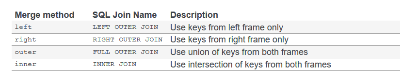
The different join types behave in the same way as they do in SQL. In Python/pandas, any missing values are shown as NaN

In order to merge the Dataframes we need to identify a column common to both of them.

PYTHON

df_cd = pd.merge(df_SN7577i_c, df_SN7577i_d, how='inner')
df_cd

In fact, if there is only one column with the same name in each Dataframe, it will be assumed to be the one you want to join on. In this example the Id column

Leaving the join column to default in this way is not best practice. It is better to explicitly name the column using the on parameter.

PYTHON

df_cd = pd.merge(df_SN7577i_c, df_SN7577i_d, how='inner', on = 'Id')

In many circumstances, the column names that you wish to join on are not the same in both Dataframes, in which case you can use the left_on and right_on parameters to specify them separately.

PYTHON

df_cd = pd.merge(df_SN7577i_c, df_SN7577i_d, how='inner', left_on = 'Id', right_on = 'Id')

Practice with data

Examine the contents of the SN7577i_aa and SN7577i_bb csv files using Excel or equivalent.
Using the SN7577i_aa and SN7577i_bb csv files, create a Dataframe which is the result of an outer join using the Id column to join on.
What do you notice about the column names in the new Dataframe?
Using shift+tab in Jupyter examine the possible parameters for the merge() function.
re-write the code so that the columns names which are common to both files have suffixes indicating the filename from which they come
If you add the parameter indicator=True, what additional information is provided in the resulting Dataframe?

Show me the solution

PYTHON

df_SN7577i_aa = pd.read_csv("SN7577i_aa.csv")
df_SN7577i_bb = pd.read_csv("SN7577i_bb.csv")
df_aabb = pd.merge(df_SN7577i_aa, df_SN7577i_bb, how='outer', on = 'Id')
df_aabb

PYTHON

df_SN7577i_aa = pd.read_csv("SN7577i_aa.csv")
df_SN7577i_bb = pd.read_csv("SN7577i_bb.csv")
df_aabb = pd.merge(df_SN7577i_aa, df_SN7577i_bb, how='outer', on = 'Id',suffixes=('_aa', '_bb'), indicator = True)
df_aabb

Key Points

You can join pandas Dataframes in much the same way as you join tables in SQL
The concat() function can be used to concatenate two Dataframes by adding the rows of one to the other.
concat() can also combine Dataframes by columns but the merge() function is the preferred way
The merge() function is equivalent to the SQL JOIN clause. ‘left’, ‘right’ and ‘inner’ joins are all possible.

Content from Wide and long data formats

Last updated on 2023-05-04 | Edit this page

Overview

Questions

What are long and Wide formats?
Why would I want to change between them?

Objectives

Explain difference between long and wide formats and why each might be used
Illustrate how to change between formats using the melt() and pivot() methods

Wide and long data formats

In the SN7577 dataset that we have been using there is a group of columns which record which daily newspapers each respondent reads. Despite the un-informative names like ‘daily1’ each column refers to a current UK daily national or local newspaper.

Whether the paper is read or not is recorded using the values of 0 or 1 as a boolean indicator. The advantage of using a column for each paper means that should a respondent read multiple newspapers, all of the required information can still be recorded in a single record.

Recording information in this wide format is not always beneficial when trying to analyse the data.

Pandas provides methods for converting data from wide to long format and from long to wide format

The SN7577 dataset does not contain a variable that can be used to uniquely identify a row. This is often referred to as a ‘primary key’ field (or column).

A dataset doesn’t need to have such a key. None of the work we have done so far has required it.

When we create a pandas Dataframe by importing a csv file, we have seen that pandas will create an index for the rows. This index can be used a bit like a key field, but as we have seen there can be problems with the index when we concatenate two Dataframes together.

In the version of SN7577 that we are going to use to demonstrate long and wide formats we will add a new variable with the name of ‘Id’ and we will restrict the other columns to those starting with the word ‘daily’.

PYTHON

import pandas as pd
df_SN7577 = pd.read_csv("SN7577.tab", sep='\t')

We will create a new Dataframe with a single column of ‘Id’.

PYTHON

# create an 'Id' column
df_papers1 = pd.DataFrame(pd.Series(range(1,1287)), index=None, columns=['Id'])

Using the range function, we can create values of Id starting with 1 and going up to 1286 (remember the second parameter to range is one past the last value used.) We have explicitly coded this value because we knew how many rows were in the dataset. If we didn’t, we could have used

PYTHON

len(df_SN7577.index) +1

{: output}

We will create a 2nd Dataframe, based on SN7577 but containing only the columns starting with the word ‘daily’.

There are several ways of doing this, we’ll cover the way that we have covered all of the prerequisites for. We will use the filter method of pandas with its like parameter.

PYTHON

df_papers2 = df_SN7577.filter(like= 'daily')

The value supplied to like can occur anywhere in the column name to be matched (and therefore selected).

Another way

If we knew the column numbers and they were all continuous we could use the iloc method and provide the index values of the range of columns we want.

PYTHON

df_papers2 = df_SN7577.iloc[:,118:143]

To create the Dataframe that we will use, we will concatenate the two Dataframes we have created.

PYTHON

df_papers = pd.concat([df_papers1, df_papers2], axis = 1)
print(df_papers.index)
print(df_papers.columns)

RangeIndex(start=0, stop=1286, step=1)
Index(['Id', 'daily1', 'daily2', 'daily3', 'daily4', 'daily5', 'daily6',
       'daily7', 'daily8', 'daily9', 'daily10', 'daily11', 'daily12',
       'daily13', 'daily14', 'daily15', 'daily16', 'daily17', 'daily18',
       'daily19', 'daily20', 'daily21', 'daily22', 'daily23', 'daily24',
       'daily25'],
      dtype='object')

{: output}

We use axis = 1 because we are joining by columns, the default is joining by rows (axis=0).

From ‘wide’ to ‘long’

To make the displays more manageable we will use only the first eight ‘daily’ columns

PYTHON

## using df_papers
daily_list = df_papers.columns[1:8]

df_daily_papers_long = pd.melt(df_papers, id_vars = ['Id'], value_vars = daily_list)

# by default, the new columns created will be called 'variable' which is the name of the 'daily'
# and 'value' which is the value of that 'daily' for that 'Id'. So, we will rename the columns

df_daily_papers_long.columns = ['Id','Daily_paper','Value']
df_daily_papers_long

We now have a Dataframe that we can groupby.

We want to groupby the Daily_paper and then sum the Value.

PYTHON

a = df_daily_papers_long.groupby('Daily_paper')['Value'].sum()
a

Daily_paper
daily1     0
daily2    26
daily3    52

{: output}

From Long to Wide

The process can be reversed by using the pivot() method. Here we need to indicate which column (or columns) remain fixed (this will become an index in the new Dataframe), which column contains the values which are to become column names and which column contains the values for the columns.

In our case we want to use the Id column as the fixed column, the Daily_paper column contains the column names and the Value column contains the values.

PYTHON

df_daily_papers_wide = df_daily_papers_long.pivot(index = 'Id', columns = 'Daily_paper', values = 'Value')

We can change our Id index back to an ordinary column with

PYTHON

df_daily_papers_wide.reset_index(level=0, inplace=True)

Exercise

Find out how many people take each of the daily newspapers by Title.
Which titles don’t appear to be read by anyone?

There is a file called Newspapers.csv which lists all of the newspapers Titles along with the corresponding ‘daily’ value

Hint: Newspapers.csv contains both daily and Sunday newspapers you can filter out the Sunday papers with the following code:

PYTHON

df_newspapers = df_newspapers[(df_newspapers.Column_name.str.startswith('daily'))]

Show me the solution

Read in Newspapers.csv file and keep only the dailies.

PYTHON

df_newspapers = pd.read_csv("Newspapers.csv")
df_newspapers = df_newspapers[(df_newspapers.Column_name.str.startswith('daily'))]
df_newspapers

Create the df_papers Dataframe as we did before.

PYTHON

import pandas as pd
df_SN7577 = pd.read_csv("SN7577.tab", sep='\t')
#create an 'Id' column
df_papers1 = pd.DataFrame(pd.Series(range(1,1287)),index=None,columns=['Id'])
df_papers2 = df_SN7577.filter(like= 'daily')
df_papers = pd.concat([df_papers1, df_papers2], axis = 1)
df_papers

Create a list of all of the dailies, one way would be

PYTHON

daily_list = []
for i in range(1,26):
    daily_list.append('daily'+str(i))

Pass the list as the value_vars parameter to the melt() method

PYTHON

#use melt to create df_daily_papers_long  
df_daily_papers_long = pd.melt(df_papers, id_vars = ['Id'], value_vars = daily_list )
#Change the column names
df_daily_papers_long.columns = ['Id', 'Daily_paper', 'Value']

merge the two Dataframes with a left join, because we want all of the Newspaper Titles to be included.

PYTHON

df_papers_taken = pd.merge(df_newspapers, df_daily_papers_long, how='left', left_on = 'Column_name',right_on = 'Daily_paper')

Then groupby the ‘Title’ and sum the ‘Value’

PYTHON

df_papers_taken.groupby('Title')['Value'].sum()

Key Points

The melt() method can be used to change from wide to long format
The pivot() method can be used to change from the long to wide format
Aggregations are best done from data in the long format.

Content from Data visualisation using Matplotlib

Last updated on 2023-05-04 | Edit this page

Overview

Questions

How can I create visualisations of my data?

Objectives

Create simple plots using pandas
Import pyplot from the matplotlib library
Customise plots using pyplot

Plotting in Python

There is a wide variety of ways to plot in Python, like many programming languages. Some do more of the design work for you and others let you customize the look of the plots and all of the little details yourself. Pandas has basic plots built into it that reduce the amount of syntax, if your data is already in a DataFrame. Matplotlib. is a Python graphical library that can be used to produce a variety of different graph types, it is fully controllable down to basic elements and includes a module pylab that is somewhere in between (designed to feel like MATLAB plotting, if you happen to have done that before).

The Matplotlib library can be imported using any of the import techniques we have seen. As Pandas is generally imported with import pandas as pd, you will find that Matplotlib is most commonly imported with import matplotlib as plt where ‘plt’ is the alias.

In addition to importing the library, in a Jupyter notebook environment we need to tell Jupyter that when we produce a graph, we want it to be display the graph in a cell in the notebook just like any other results. To do this we use the %matplotlib inline directive.

Although we are using Matplotlib in this episode, Pandas can make use of several other graphical libraries available from within Python such as ggplot2 and Seaborn. Seaborn has some very powerful features and advanced plot types. One of its most useful features is formatting.

Plotting with Pandas

The Pandas library contains very tight integration with Matplotlib. There are functions in Pandas that automatically call Matplotlib functions to produce graphs.

To plot with Pandas we have to import it as we have done in past episodes. To tell Jupyter that when we produce a graph we want it to be displayed in a cell in the notebook just like any other results, we use the %matplotlib inline directive. Without that we need to do a show() command.

PYTHON

import pandas as pd
%matplotlib inline

We also need data to work with loaded into a DataFrame and it’s helpful to look at a few rows to remember what’s there.

We are going to use the dataset from the setup page, SAFI_full_shortname.csv. For the data to load, make sure to have that file in the same folder where your Jupyter notebook is running. If the file is not in that folder, you are going to have to type the full path.

PYTHON

df = pd.read_csv("SAFI_full_shortname.csv")
df.head()

Next, we can plot the a histogram of a variable.

PYTHON

df['years_liv'].hist()

Histogram of years lived spotlighting how to plot a variable with Pandas

We can change the number of bins to make it look how we would like, for example

PYTHON

df['years_liv'].hist(bins=20)

We can also specify the column as a parameter and a groupby column with the by keyword. there are a lot of keywords available to make it look better, we can see some of the most likely ones (as decided by Pandas developers) by using shift + tab .

Lets try layout, figsize, and sharex.

PYTHON

df.hist(column='years_liv',by='village',layout=(1,3),figsize=(12,3),sharex=True)

Three separate histograms depicting the number of years lived by village; Chirodzo, God, Ruaca

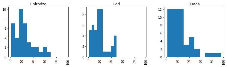
Scatter plot

The scatter plot requires the x and y coordinates of each of the points being plotted. We can add a third dimension as different colors with the c argument.

PYTHON

df.plot.scatter(x='gps_Latitude', y='gps_Longitude', c='gps_Altitude', colormap="viridis", figsize=[4,4])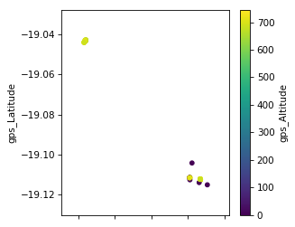

Exercise

Make a scatter plot of years_farm vs years_liv and color the points by buildings_in_compound
Make a bar plot of the mean number of rooms per wall type

Compare the two graphs we have just drawn. How do they differ? Are the differences significant?

Show me the solution

Most importantly the data in the graphs is the same. There are cosmetic differences in the scale points in the x and y axis and in the width of the bars.

The width of the bars can be changed with a parameter in the ‘bar’ function

PYTHON

plt.bar(range(len(s)), s, width = 0.5)   # the default width is 0.8

Extension: try plotting by wall and roof type?

Show me the solution

For the scatter plot:

PYTHON

df.plot.scatter(x = 'years_liv', y = 'years_farm', c = 'buildings_in_compound', colormap = 'viridis')

For the barplot: we first need to calculate the mean value of rooms per wall type, then we can make the plot.

PYTHON

rooms_mean = df.groupby('respondent_wall_type').mean()['rooms']
rooms_mean.plot.bar()

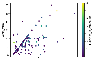
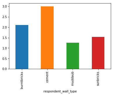
Boxplot

A boxplot provides a simple representation of a variety of statistical qualities of a single set of data values. A common use of the boxplot is to compare the statistical variations across a set of variables.

The variables can be an independent series or columns of a Dataframe using the Pandas plot method

df.boxplot(by ='village',column=['buildings_in_compound'])

{:.language-python}

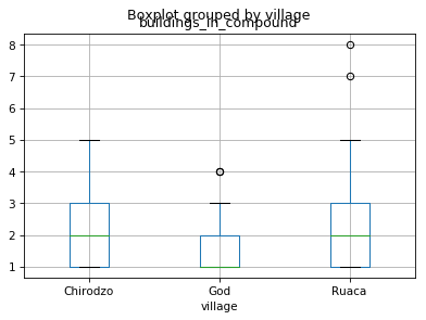
We can make it look prettier with Seaborn, much more easily than fixing components manually with Matplotlib. Seaborn is a Python data visualization library based on Matplotlib. It provides a high-level interface for drawing attractive and informative statistical graphics. Seaborn comes with Anaconda; to make it available in our Python session we need to import it.

PYTHON

import seaborn as sns
sns.boxplot(data = df, x = 'village', y = 'buildings_in_compound')

We can also draw linear models in a plot using lmplot() from seaborn, e.g. for years_farm vs years_liv per village.

PYTHON

sns.lmplot(x='years_farm', y='years_liv',data=df,hue='village')

Plot showing years lived and years farmed by village to spotlight the use of linear models

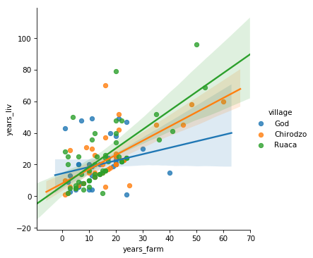
In general, most graphs can be broken down into a series of elements which, although typically related in some way, can all exist independently of each other. This allows us to create the graph in a rather piecemeal fashion.

The labels (if any) on the x and y axis are independent of the data values being represented. The title and the legend are also independent objects within the overall graph.

In Matplotlib you create the graph by providing values for all of the individual components you choose to include. When you are ready, you call the show function.

Using this same approach, we can plot two sets of data on the same graph.

We will use a scatter plot to demonstrate some of the available features.

Fine-tuning figures with Matplotlib

If we want to do more advanced or lower level things with our plots, we need to use Matplotlib directly, not through Pandas. First we need to import it.

Customising our plots with Matplotlib

We can further customise our plots with Matplotlib directly. First we need to import it. The Matplotlib library can be imported using any of the import techniques we have seen. As Pandas is generally imported with import pandas as pd, you will find that matplotlib is most commonly imported with import matplotlib.pyplot as plt where plt is the alias. For demonstration purposes, we are going to use randomly generated data, using the NumPy library (aliased here as np).

PYTHON

import numpy as np
import pandas as pd
import matplotlib.pyplot as plt

# Generate some date for 2 sets of points.
x1 = pd.Series(np.random.rand(20) - 0.5)
y1 = pd.Series(np.random.rand(20) - 0.5)

x2 = pd.Series(np.random.rand(20) + 0.5)
y2 = pd.Series(np.random.rand(20) + 0.5)


# Add some features
plt.title('Scatter Plot')
plt.ylabel('Range of y values')
plt.xlabel('Range of x values')

# plot the points in a scatter plot
plt.scatter(x1, y1, c='red', label='Red Range')  # 'c' parameter is the colour and 'label' is the text for the legend
plt.scatter(x2, y2, c='blue', label='Blue Range')

plt.legend(loc=4)  # the locations 1,2,3 and 4 are top-right, top-left, bottom-left and bottom-right
# Show the graph with the two sets of points
plt.show()

In the call to the scatter method, the label parameter values are used by the legend. The c or color parameter can be set to any color Matplotlib recognises. Full details of the available colours are available in the Matplotlib website. The markers section will tell you what markers you can use instead of the default ‘dots’. There is also an s (size) parameter which allows you to change the size of the marker.

Exercise

In the scatterplot the s parameter determines the size of the dots. s can be a simple numeric value, say s=100, which will produce dots all of the same size. However, you can pass a list of values (or a Pandas Series) to provide sizes for the individual dots. This approach is very common as it allows us to provide an extra variable worth of information on the graph.

Modify the code we used for the scatter plot to include a size value for each of the points in the series being plotted. (The downside is that some of the smaller dots may be completely covered by the larger dots. To try and highlight when this has happened, we can change the opacity of the dots.)
Find out which parameter controls the opacity of the dots (clue - it is not called opacity), add it to you code and set it > to a reasonable value.

Show me the solution

PYTHON

# Generate some data for 2 sets of points.
# and additional data for the sizes - suitably scaled
x1 = pd.Series(np.random.rand(20) - 0.5)
y1 = pd.Series(np.random.rand(20) - 0.5)
z1 = pd.Series(np.random.rand(20) * 200)

x2 = pd.Series(np.random.rand(20) + 0.5)
y2 = pd.Series(np.random.rand(20) + 0.5)
z2 = pd.Series(np.random.rand(20) * 200)

# Add some features
plt.title('Scatter Plot')
plt.ylabel('Range of y values')
plt.xlabel('Range of x values')

# plot the points in a scatter plot
plt.scatter(x1, y1, c='red', label='Red Range', s=z1, alpha=0.5)  # 's' parameter is the dot size
plt.scatter(x2, y2, c='blue', label='Blue Range', s=z2, alpha=0.5) # 'alpha' is the opacity

plt.legend(loc=4)
plt.show()

Internally the Pandas ‘plot’ method has called the ‘bar’ method of Matplotlib and provided a set of parameters, including the pandas.Series s to generate the graph.

We can use Matplotlib directly to produce a similar graph. In this case we need to pass two parameters, the number of bars we need and the Pandas Series holding the values.

Let’s redo the boxplot we did above:

PYTHON

df.boxplot(column = 'buildings_in_compound', by = 'village')

The automatic title of the plot does not look good, we are missing a title for the y-axis and we do not need the extra x-axis title. We can also remove the gridlines. Let’s fix these things using functions from plt. Note: all the adjustments for the plot have to go into the same notebook cell together with the plot statement itself.

PYTHON

df.boxplot(column = 'buildings_in_compound', by = 'village')
plt.suptitle('') # remove the automatic title
plt.title('Buildings in compounds per village')   # add a title
plt.ylabel('Number of buildings')   # add a y-axis title
plt.xlabel('')   # remove the x-axis title
plt.grid(None)   # remove the grid lines

In general most graphs can be broken down into a series of elements which, although typically related in some way, can all exist independently of each other. This allows us to create the graph in a rather piecemeal fashion. The labels (if any) on the x and y axis are independent of the data values being represented. The title and the legend are also independent objects within the overall graph. In matplotlib you create the graph by providing values for all of the individual components you choose to include.

Saving a graph

If you wish to save your graph as an image you can do so using the plt.savefig() function. The image can be saved as a pdf, jpg or png file by changing the file extension. plt.savefig() needs to be called at the end of all your plot statements in the same notebook cell.

PYTHON

df.boxplot(column = 'buildings_in_compound', by = 'village')
plt.suptitle('') # remove the automatic title
plt.title('Buildings in compounds per village')   # add a title
plt.ylabel('Number of buildings')   # add a y-axis title
plt.xlabel('')   # remove the x-axis title
plt.grid(None)   # remove the grid lines
plt.savefig('safi_boxplot_buildings.pdf')   # save as pdf file
plt.savefig('safi_boxplot_buildings.png', dpi = 150)  # save as png file, some extra arguments are provided

The labels (if any) on the x and y axis are independent of the data values being represented. The title and the legend are also independent objects within the overall graph.

In Matplotlib you create the graph by providing values for all of the individual components you choose to include. When you are ready, you call the show function.

Using this same approach we can plot two sets of data on the same graph. We will use a scatter plot to demonstrate some of the available features.

Exercise

Revisit your favorite plot we’ve made so far, or make one with your own data then:

add axes labels
add a title
add a legend
save it in two different formats

extension: try plotting by wall and roof type!

Key Points

Graphs can be drawn directly from Pandas, but it still uses Matplotlib
Different graph types have different data requirements
Graphs are created from a variety of discrete components placed on a ‘canvas’, you don’t have to use them all

Content from Accessing SQLite Databases

Last updated on 2023-05-04 | Edit this page

Overview

Questions

How can I access database tables using Pandas and Python?
What are the advantages of storing data in a database

Objectives

Use the sqlite3 module to interact with a SQL database
Access data stored in SQLite using Python
Describe the difference in interacting with data stored as a CSV file versus in SQLite
Describe the benefits of accessing data using a database compared to a CSV file

Introducing the sqlite3 module

SQLite is a relational database system. Despite the ‘Lite’ in the name it can handle databases in excess of a Terabyte. The ‘Lite’part really relates to the fact that it is a ’bare bones’ system. It provides the mechanisms to create and query databases via a simple command line interface but not much else. In the SQL lesson we used a Firefox plugin to provide a GUI (Graphical User Interface) to the SQLite database engine.

In this lesson we will use Python code using the sqlite3 module to access the engine. We can use Python code and the sqlite3 module to create, delete and query database tables.

In practice we spend a lot of the time querying database tables.

Pandas Dataframe v SQL table

It is very easy and often very convenient to think of SQL tables and pandas Dataframes as being similar types of objects. All of the data manipulations, slicing, dicing, aggragetions and joins associated with SQL and SQL tables can all be accomplished with pandas methods operating on a pandas Dataframe.

The difference is that the pandas Dataframe is held in memory within the Python environment. The SQL table can largely be on disc and when you access it, it is the SQLite database engine which is doing the work. This allows you to work with very large tables which your Python environment may not have the memory to hold completely.

A typical use case for SQLite databases is to hold large datasets, you use SQL commands from Python to slice and dice and possibly aggregate the data within the database system to reduce the size to something that Python can comfortably process and then return the results to a Dataframe.

Accessing data stored in SQLite using Python

We will illustrate the use of the sqlite3 module by connecting to an SQLite database using both core Python and also using pandas.

The database that we will use is SN7577.sqlite This contains the data from the SN7577 dataset that we have used in other lessons.

Connecting to an SQlite database

The first thing we need to do is import the sqlite3 library, We will import pandas at the same time for convenience.

PYTHON

import sqlite3
import pandas as pd

We will start looking at the sqlite3 library by connecting to an existing database and returning the results of running a query.

Initially we will do this without using Pandas and then we will repreat the exercise so that you can see the difference.

The first thing we need to do is to make a connection to the database. An SQLite database is just a file. To make a connection to it we only need to use the sqlite3 connect() function and specify the database file as the first parameter.

The connection is assigned to a variable. You could use any variable name, but ‘con’ is quite commonly used for this purpose

PYTHON

con = sqlite3.connect('SN7577.sqlite')

The next thing we need to do is to create a cursor for the connection and assign it to a variable. We do this using the cursor method of the connection object.

The cursor allows us to pass SQL statements to the database, have them executed and then get the results back.

To execute an SQL statement we use the execute() method of the cursor object.

The only paramater we need to pass to execute() is a string which contains the SQL query we wish to execute.

In our example we are passing a literal string. It could have been contained in a string variable. The string can contain any valid SQL query. It could also be a valid DDL statement such as a “CREATE TABLE …”. In this lesson however we will confine ourseleves to querying exiting database tables.

PYTHON

cur = con.cursor()
cur.execute("SELECT * FROM SN7577")

<sqlite3.Cursor at 0x115e10d50>

{: output}

The execute() method doesn’t actually return any data, it just indicates that we want the data provided by running the SELECT statement.

Exercise

What happens if you if you ask for a non existent table?, field within a table? or just any kind of syntax error?

Show me the solution

PYTHON

cur = con.cursor()
# notice the mistyping of 'SELECT'
cur.execute("SELET * FROM SN7577")

In all cases an error message is returned. The error message is not from Python but from SQLite. It is the same error message that you would have got had you made the same errors in the SQLite plugin.

Before we can make use of the results of the query we need to use the fetchall() method of the cursor.

The fetchall() method returns a list. Each item in the list is a tuple containing the values from one row of the table. You can iterate through the items in a tuple in the same way as you would do so for a list.

PYTHON

cur = con.cursor()
cur.execute("SELECT * FROM SN7577")
rows = cur.fetchall()
for row in rows:
    print(row)

(1, -1, 1, 8, 0, 0, 0, 1, 0, 0, 0, 0, 0, 0, 0, 0, 0, 0, 0, 1, 0, 0, 1, 0, 0, 1, 0, 0, 0, 0, 0, 0, 0, 0, 3, 3, 3, 2, 3, 3, 4, 1, 4, 2, 2, 2, 2, 1, 0, 0, 0, 3, 2, 3, 3, 1, 4, 2, 3
...

{: output}

The output is the data only, you do not get the column names.

The column names are available from the ‘description’ of the cursor.

PYTHON

colnames = []
for description in cur.description :
    colnames.append(description[0])

print(colnames)

['Q1', 'Q2', 'Q3', 'Q4', 'Q5ai', 'Q5aii', 'Q5aiii', 'Q5aiv', 'Q5av', 'Q5avi', 'Q5avii', 'Q5aviii', 'Q5aix', 'Q5ax', 'Q5axi', 'Q5axii', 'Q5axiii', 'Q5axiv', 'Q5axv', 'Q5bi', 'Q5bii', 'Q5biii', 'Q5biv', 'Q5bv', 'Q5bvi', 'Q5bvii', 'Q5bviii', 'Q5bix', 'Q5bx', 'Q5bxi', 'Q5bxii', 'Q5bxiii', 'Q5bxiv', 'Q5bxv', 'Q6', 'Q7a', 'Q7b', 'Q8', 'Q9', 'Q10a', 'Q10b', 'Q10c', 'Q10d', 'Q11a',
...

{: output}

One reason for using a database is the size of the data involved. Consequently it may not be practial to use fetchall() as this will return the complete result of your query.

An alternative is to use the fetchone() method, which as the name suggestrs returns only a single row. The cursor keeps track of where you are in the results of the query, so the next call to fetchone() will return the next record. When there are no more records it will return ‘None’.

PYTHON

cur = con.cursor()
cur.execute("SELECT * FROM SN7577")
row = cur.fetchone()
print(row)
row = cur.fetchone()
print(row)

(1, -1, 1, 8, 0, 0, 0, 1, 0, 0, 0, 0, 0, 0, 0, 0, 0, 0, 0, 1, 0, 0, 1, 0, 0, 1, 0, 0, 0, 0, 0, 0, 0, 0, 3, 3, 3, 2, 3, 3, 4, 1, 4, 2, 2, 2, 2, 1, 0, 0, 0, 3, 2, 3, 3, 1, 4, 2, 3, 2, 4, 4, 2, 2, 2, 4, 2, 1, 1, 0, 1, 0, 0, 1, 0, 0, 0, 1, 0, 0, 0, 0, 0, 0, 0, 0

{: output}

Exercise

Can you write code to return the first 5 records from the SN7577 table in two different ways?

Show me the solution

PYTHON

import sqlite3
con = sqlite3.connect('SN7577.sqlite')
cur = con.cursor()

# we can use the SQLite 'limit' clause to restrict the number of rows returned and then use 'fetchall'
cur.execute("SELECT * FROM SN7577 Limit 5")
rows = cur.fetchall()

for row in rows:
    print(row)

# we can use 'fetchone' in a for loop
cur.execute("SELECT * FROM SN7577")
for i in range(1,6):
    print(cur.fetchone())

# a third way would be to use the 'fetchmany()' method

cur.execute("SELECT * FROM SN7577")
rows = cur.fetchmany(5)

for row in rows:
    print(row)

Using Pandas to read a database table.

When you use Pandas to read a database table, you connect to the database in the same way as before using the SQLite3 connect() function and providing the filename of the database file.

Pandas has a method read_sql_query to which you provide both the string containing the SQL query you wish to run and also the connection variable.

The results from running the query are placed in a pandas Dataframe with the table column names automatically added.

PYTHON

con = sqlite3.connect('SN7577.sqlite')
df = pd.read_sql_query("SELECT * from SN7577", con)

# verify that result of SQL query is stored in the Dataframe
print(type(df))
print(df.shape)
print(df.head())

con.close()

Saving a Dataframe as an SQLite table

There may be occasions when it is convenient to save the data in you pandas Dataframe as an SQLite table for future use or for access to other systems. This can be done using the to_sql() method.

PYTHON

con = sqlite3.connect('SN7577.sqlite')
df = pd.read_sql_query("SELECT * from SN7577", con)

# select only the row where the response to Q1 is 10 meaning undecided voter
df_undecided = df[df.Q1 == 10]
print(df_undecided.shape)

# Write the new Dataframe to a new SQLite table
df_undecided.to_sql("Q1_undecided", con)

# If you want to overwrite an existing SQLite table you can use the 'if_exists' parameter
#df_undecided.to_sql("Q1_undecided", con, if_exists="replace")
con.close()

(335, 202)

{: output}

Deleting an SQLite table

If you have created tables in an SQLite database, you may also want to delete them. You can do this by using the sqlite3 cursor execute() method

PYTHON

con = sqlite3.connect('SN7577.sqlite')
cur = con.cursor()

cur.execute('drop table if exists Q1_undecided')

con.close()

Exercise

The code below creates an SQLite table as we have done in previous examples. Run this code to create the table.

con = sqlite3.connect('SN7577.sqlite')
df_undecided = df[df.Q1 == 10]
df_undecided.to_sql("Q1_undecided_v2", con)
con.close()

Try using the following pandas code to delete (drop) the table.

PYTHON

pd.read_sql_query("drop table Q1_undecided_v2", con)

What happens?
Run this line of code again, What is different?
Can you explain the difference and does the table now exist or not?

Show me the solution

When the line of code is run the first time you get an error message : ‘NoneType’ object is not iterable.
When you run it a second time you get a different error message: DatabaseError: Execution failed on sql ‘drop table Q1_undecided_v2’: no such table: Q1_undecided_v2
the read_sql_query() method is designed to send the SQL containing your query to the SQLite execution engine, which will execute the SQL and return the output to pandas which will create a Dataframe from the results.

The SQL statement we sent is valid SQL but it doesn’t return rows from a table, it simply reports success of failure (in dropping the table in this case). The first time we run it the table is deleted and a response to the effect is returned. The resonse cannot be converted to a Dataframe, hence the first error message, which is a pandas error.

When we run it for the second time, the table has already has already been dropped, so this time the error message is from SQLite saying the table didn’t exist. Pandas recognises that this is an SQLite error message and simply passes it on to the user.

The moral of the story: pandas may be better for getting data returned into a Dataframe, but there are some things best left to the sqlite functions directly.

Key Points

The SQLite database system is directly available from within Python
A database table and a pandas Dataframe can be considered similar structures
Using pandas to return all of the results from a query is simpler than using sqlite3 alone