Learning Objectives
Following this assignment students should be able to:
- use and create vectorized functions
- use the apply family of functions for iteration
- integrate custom functions with dplyr for iteration
Reading
-
Topics
- Iteration
- Style
-
Readings
Lecture Notes
Setup
install.packages(c('dplyr', 'ggplot2', 'readr', 'tidyr'))
download.file("https://datacarpentry.org/semester-biology/data/dinosaur_lengths.csv",
  "dinosaur_lengths.csv")
download.file("https://datacarpentry.org/semester-biology/data/ramesh2010-macroplots.csv",
  "ramesh2010-macroplots.csv")
download.file("https://ndownloader.figshare.com/files/5629536",
  "TREE_SURVEYS.txt")
download.file("https://ndownloader.figshare.com/files/2292172",
  "surveys.csv")
download.file("https://ndownloader.figshare.com/files/3299474",
  "plots.csv")
download.file("https://ndownloader.figshare.com/files/3299483",
  "species.csv")
Lecture Notes
Place this code at the start of the assignment to load all the required packages.
library(dplyr)
library(ggplot2)
Exercises
Size Estimates Vectorized (10 pts)
The length of an organism is typically strongly correlated with its body mass. This is useful because it allows us to estimate the mass of an organism even if we only know its length. This relationship generally takes the form:
mass = a * lengthb
Parameters
aandbvary among groups.-
Write a function named
mass_from_length_theropoda()that takeslengthas an argument to get an estimate of mass values for the dinosaur Theropoda. Use the equationmass <- 0.73 * length^3.63. Copy the data below into R and pass the entire vector to your function to calculate the estimated mass for each dinosaur.theropoda_lengths <- c(17.8013631070471, 20.3764452071665, 14.0743486294308, 25.65782386974, 26.0952008049675, 20.3111541103134, 17.5663244372533, 11.2563431277577, 20.081903202614, 18.6071626441984, 18.0991894513166, 23.0659685685892, 20.5798853467837, 25.6179254233558, 24.3714331573996, 26.2847248252537, 25.4753783544473, 20.4642089867304, 16.0738256364701, 20.3494171706583, 19.854399305869, 17.7889814608919, 14.8016421998303, 19.6840911485379, 19.4685885050906, 24.4807784966691, 13.3359960054899, 21.5065994598917, 18.4640304608411, 19.5861532398676, 27.084751999756, 18.9609366301798, 22.4829168046521, 11.7325716149514, 18.3758846100456, 15.537504851634, 13.4848751773738, 7.68561192214935, 25.5963348603783, 16.588285389794) -
Create a new version of the function named
mass_from_length()to use the equationmass <- a * length^band takelength,aandbas arguments. In the function arguments, set the default values forato0.73andbto3.63. If you run this function with just the length data from Part 1, you should get the same result as Part 1. Copy the data below into R and call your function using the vector of lengths from Part 1 (above) and these vectors ofaandbvalues to estimate the mass for the dinosaurs using different values ofaandb.a_values <- c(0.759, 0.751, 0.74, 0.746, 0.759, 0.751, 0.749, 0.751, 0.738, 0.768, 0.736, 0.749, 0.746, 0.744, 0.749, 0.751, 0.744, 0.754, 0.774, 0.751, 0.763, 0.749, 0.741, 0.754, 0.746, 0.755, 0.764, 0.758, 0.76, 0.748, 0.745, 0.756, 0.739, 0.733, 0.757, 0.747, 0.741, 0.752, 0.752, 0.748)b_values <- c(3.627, 3.633, 3.626, 3.633, 3.627, 3.629, 3.632, 3.628, 3.633, 3.627, 3.621, 3.63, 3.631, 3.632, 3.628, 3.626, 3.639, 3.626, 3.635, 3.629, 3.642, 3.632, 3.633, 3.629, 3.62, 3.619, 3.638, 3.627, 3.621, 3.628, 3.628, 3.635, 3.624, 3.621, 3.621, 3.632, 3.627, 3.624, 3.634, 3.621) -
Create a data frame for this data using
dino_data <- data.frame(theropoda_lengths, a_values, b_values). Usedplyrto add a newmassescolumn to this data frame (usingmutate()and your function) and print the result to the console.
-
Size Estimates With Maximum (10 pts)
Write a function named named
mass_from_length_maxthat takeslengthas an argument. Iflengthis less than 20 estimate the mass of the dinosaur using the equationmass <- 0.73 * length ^ 3.63. Iflengthis greater than or equal to 20 returnNAinstead.Copy the data below into R and use
sapply()and this new function to estimate the mass for every length indinosaur_lengths.Expected outputs for Size Estimates With Maximumdinosaur_lengths <- c(17.8013631070471, 20.3764452071665, 14.0743486294308, 25.65782386974, 26.0952008049675, 20.3111541103134, 17.5663244372533, 11.2563431277577, 20.081903202614, 18.6071626441984, 18.0991894513166, 23.0659685685892, 20.5798853467837, 25.6179254233558, 24.3714331573996, 26.2847248252537, 25.4753783544473, 20.4642089867304, 16.0738256364701, 20.3494171706583, 19.854399305869, 17.7889814608919, 14.8016421998303, 19.6840911485379, 19.4685885050906, 24.4807784966691, 13.3359960054899, 21.5065994598917, 18.4640304608411, 19.5861532398676, 27.084751999756, 18.9609366301798, 22.4829168046521, 11.7325716149514, 18.3758846100456, 15.537504851634, 13.4848751773738, 7.68561192214935, 25.5963348603783, 16.588285389794)Size Estimates By Name Apply (20 pts)
If the data on dinosaur lengths with species names is not in your working directory then download it. Import it using
read_csv().The following function estimates a dinosaur’s mass based on its length and name of its taxonomic group:
get_mass_from_length_by_name <- function(length, name){ if (name == "Stegosauria"){ mass = 10.95 * length ^ 2.64 } else if (name == "Theropoda"){ mass = 0.73 * length ^ 3.63 } else if (name == "Sauropoda"){ mass = 214.44 * length ^ 1.46 } else { mass = NA } return(mass) }-
Copy this function into your code and then use this function and
mapply()to calculate the estimated mass for each dinosaur. You’ll need to pass the data tomapply()as single vectors or columns, not the whole data frame. -
Using
dplyr, add a newmassescolumn to the data frame (usingrowwise(),mutate()and your function) and print the result to the console. -
Using
ggplot, make a histogram of dinosaur masses with one subplot for each species (usingfacet_wrap()).
-
Crown Volume Calculation (25 pts)
The UHURU experiment in Kenya has conducted a survey of Acacia and other tree species in ungulate exclosure treatments. If
TREE_SURVEYS.txtis not on in your working directory then download a copy. Each of the individuals surveyed were measured for tree height (HEIGHT) and canopy size in two directions (AXIS_1andAXIS_2). Read these data in using the following code:tree_data <- read_tsv("TREE_SURVEYS.txt", na = c("dead", "missing", "MISSING", "NA", "?", "3.3."))You want to estimate the crown volumes for the different species and have developed equations for species in the Acacia genus:
volume <- 0.16 * HEIGHT ^ 0.8 * pi * AXIS_1 * AXIS_2and the Balanites genus:
volume <- 1.2 * HEIGHT ^ 0.26 * pi * AXIS_1 * AXIS_2For all other genera you’ll use a general equation developed for trees:
volume <- 0.5 * HEIGHT ^ 0.6 * pi * AXIS_1 * AXIS_2-
Write a function called
tree_volume_calcthat calculates the canopy volume for the Acacia species in the dataset. To do so, use an if statement in combination with thestr_detect()function from thestringrR package. The codestr_detect(SPECIES, "Acacia")will returnTRUEif the string stored in this variable contains the word “Acacia” andFALSEif it does not. This function will have to take the following arguments as input: SPECIES, HEIGHT, AXIS_1, AXIS_2. Then run the following line:tree_volume_calc("Acacia_brevispica", 2.2, 3.5, 1.12) -
Expand this function to additionally calculate canopy volumes for other types of trees in this dataset by adding if/else statements and including the volume equations for the Balanites genus and other genera. Then run the following lines:
tree_volume_calc("Balanites", 2.2, 3.5, 1.12)tree_volume_calc("Croton", 2.2, 3.5, 1.12) -
Now get the canopy volumes for all the trees in the
tree_datadataframe and add them as a new column to the data frame. You can do this usingtree_volume_calc()and eithermapply()or usingdplyrwithrowwiseandmutate.
-
Portal Data Iteration Without Loops (25 pts)
This exercise covers iteration without loops in R using Portal data. You’ll practice vectorization, apply functions, and integration with dplyr using real ecological data from the Portal Project.
If surveys.csv, species.csv, and plots.csv are not in your working directory then download them.
Load the three data files using
read_csv.1. Create a vectorized function called
estimate_metabolic_ratethat takesweightas input and returns metabolic rate using the equation:metabolic_rate = 0.073 * weight ^ 0.75. Run it on the following vector:weights <- c(15, 25, 35, 45, 20, 70, 72).2. Use
mutate()andestimate_metabolic_rateto create a version of the data insurveyswith a column calledmetabolic_ratefor all animals that have weight measurements. Remove the rows without metabolic rates. Select theyear,species_id, andmetabolic_ratecolumns.3. Create a function called
classify_by_weightthat takes a single weight value and returns:- “small” if weight < 20g
- “medium” if weight is 20-50g
- “large” if weight > 50g
- “unknown” if weight is missing (
NA)
Use
sapplyto applyclassify_by_weightto theweightsvector from (1).4. Use
mutate,classify_by_weight, and thesurveystable to produce a data frame that has data on theyear,plot_id,species_id, andweight_class(whereweight_classis the output ofclassify_by_weight). Join this data with theplotstable to add information onplot_type. Filter the data to only include data whereplot_typeis “Control”.5. Group the results of (4) based on
plot_idandweight_class(usinggroup_by) and count the number of individuals in each group (usingsummarize).6. Create a function called
energy_budget()that takesgenus,species, andweightas inputs (you’ll need to join thesurveysandspeciestables to get this data together). It should return daily energy needs for each individual in surveys based on the values ofgenusandspeciesusing the following equations:- If
genusis “Dipodomys” :energy = 0.065 * avg_weight ^ 0.75 * 24 - If
genusis “Chaetodipus” andspeciesis “penicillatus”:energy = 0.080 * avg_weight ^ 0.75 * 24 - If
genusis “Chaetodipus” andspeciesis “baileyi”:energy = 0.26 * avg_weight ^ 0.75 * 24 - All other species:
energy = 0.073 * avg_weight ^ 0.75 * 24
Run the function with
mapply()and the following inputs:genus:c("Dipodomys", "Chaetodipus", "Neotoma")species:c("merriami", "penicillatus", "albigula")weight:c(45, 22, 156)
7. Use
Expected outputs for Portal Data Iteration Without Loopsmutateandrowwiseto calculate energy budget for each individual insurveys. Drop rows withNAfor the newenergy_budgetcolumn. Group and summarize the data to get an total energy budget for each combination ofyear,month, anddayby summing all of the values ofenergy_budgetin each group.Check That Your Code Runs (10 pts)
Sometimes you think you’re code runs, but it only actually works because of something else you did previously. To make sure it actually runs you should save your work and then run it in a clean environment.
Follow these steps in RStudio to make sure your code really runs:
1. Restart R (see above) by clicking
Sessionin the menu bar and selectingRestart R: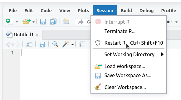
2. If the
Environmenttab isn’t empty click on the broom icon to clear it:
The
Environmenttab should now say “Environment Is Empty”: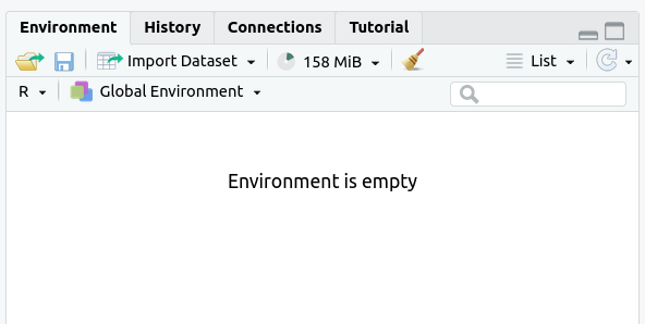
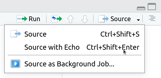
3. Rerun your entire homework assignment using “Source with Echo” to make sure it runs from start to finish and produces the expected results.
4. Make sure that you saved your code with the name
assignmentsomewhere in the file name. You should see the file in theFilestab and the name of the file should be black (not red with an*in the tab at the top of the text editor):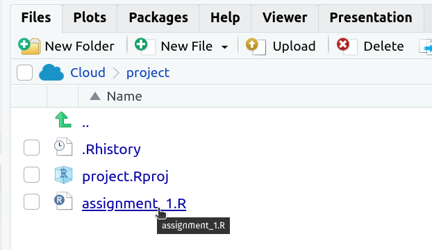

5. Make sure that your code will run on other computers
- No
setwd()(use RStudio Projects instead) - Use
/not\for paths
- No
Tree Growth (Challenge - optional)
The UHURU experiment in Kenya has conducted a survey of Acacia and other tree species in ungulate exclosure treatments. Each of the individuals surveyed were measured for tree height (
HEIGHT), circumference (CIRC) and canopy size in two directions (AXIS_1andAXIS_2). If the fileTREE_SURVEYS.txtisn’t already in your working directory, download the data file here.Read the data in using the following code:
tree_data <- read_tsv("TREE_SURVEYS.txt", na = c("dead", "missing", "MISSING", "NA", "?", "3.3."))-
Write a function named
get_growth()that takes two inputs, a vector ofsizesand a vector ofyears, and calculates the average annual growth rate. Pseudo-code for calculating this rate is(size_in_last_year - size_in_first_year) / (last_year - first_year). Test this function by runningget_growth(c(40.2, 42.6, 46.0), c(2020, 2021, 2022)). -
Use dplyr and this function to get the growth for each individual tree along with information about the
TREATMENTthat tree occurs on. Trees are identified by a unique value in theORIGINAL_TAGcolumn. Don’t include information for cases where aTREATMENTis not known (e.g., where it isNA). -
Using ggplot and the output from (2) make a histogram of growth rates for each
TREATMENT, which eachTREATMENTin it’s own facet. Usegeom_vline()to add a vertical line at 0 to help indicate which trees are getting bigger vs. smaller. Include good axis labels. -
Create a single function called
compare_growth()that combines your work in (2) and (3). It should take the arguments:df(the data frame being used),measure(the column that contains the size measurement to measure growth on; we usedCIRC),tag_column(the name of the column with the unique tag; we usedORIGINAL_TAG),sample_column(the name of the column indicating different samples, we usedYEAR), andfacet_column(the name of the column to use to determine which groups to make histograms for, we usedTREATMENT). Use the function to recreate your original plot usingcompare_growth(tree_data, CIRC, ORIGINAL_TAG, YEAR, TREATMENT). Then use the function to create a similar plot showing growth facetedSPECIES, usingSURVEYas thesample_column, andAXIS_1as themeasureby runningcompare_growth(tree_data, AXIS_1, ORIGINAL_TAG, SURVEY, SPECIES).
-