Learning Objectives
Following this assignment students should be able to:
- import, view properties, and plot a
raster- perform simple
rastermath- import, view properties, and plot vector data
- extract points from a
rasterusing a shapefile
Reading
Lecture Notes
Setup
install.packages(c("dplyr", "ggplot2", "sf", "terra", "tidyterra"))
download.file("www.datacarpentry.org/semester-biology/data/neon-geospatial-data.zip", "neon-geospatial-data.zip", mode = "wb")
unzip("neon-geospatial-data.zip")
file.rename("neon-geospatial-data/", "data/")
Lectures
- Spatial Data Raster
- Spatial Data Raster Math
- Spatial Data Vector
- Spatial Data Projections
- Spatial Data Extracting Raster Values
Place this code at the start of the assignment to load all the required packages.
library(terra)
library(tidyterra)
library(sf)
library(ggplot2)
library(dplyr)
Exercises
Canopy Height from Space (90 pts)
The National Ecological Observatory Network has invested in high-resolution airborne imaging of their field sites. Elevation models generated from LiDAR can be used to map the topography and vegetation structure at the sites.
Check to see if there is a
datadirectory in your workspace with anSJERsubdirectory in it. If not, Download the data and extract it into your working directory. TheSJERdirectory contains raster data for a digital terrain model (sjer_dtmcrop.tif) and a digital surface model (sjer_dsmcrop.tif), and vector data on plot locations (sjer_plots.shp) and the site boundary (sjer_boundar.shp) for the San Joaquin Experimental Range.- Map the digital terrain model for
SJERusing theviridiscolor ramp. - Create and map the canopy height model for
SJERusing theviridiscolor ramp. To do this subtract the values in the digital terrain model from the values in the digital surface model usingrastermath (chm = dsm - dtm). - Create a map that shows the
SJERboundary and the plot locations colored byplot_type. - Transform the plot data to have the same CRS as the CHM. Show CRS for both objects. Create a map that shows the canopy height model from (3) with the plot locations on top.
- Extract the canopy heights at each plot location for
SJERand display the values. - Building on (5) create a version of your code that extracts the canopy heights and includes them with the data in
plots_sjer_utm. You can do this using eithermutate(to add the results of (5) toplots_sjer_utmorbindput the data together inextractandst_as_sfto convert the resulting terra object into a simple features object. Display the full simple features object. Make sure that the column name for the canopy heights iscanopy_height. The detailed display will vary depending on your approach. - Create a map that shows the
SJERboundary and the plot locations colored by the canopy height values. - Create a map that shows the canopy height model raster, but in
cmrather thanm(i.e., multiply the canopy height model by 100). - Create a map that shows the digital terrain model raster, the plot locations, and the
SJERboundary, using transparency as needed to allow all three layers to be seen. Remember all three layers will need to have the same CRS. - Conduct an analysis of the relationship between elevation and canopy height at the SJER plots. Using a 50m buffer, extract the mean elevations (i.e., the values from the digital terrain model) and the canopy heights at each plot location for
SJERand add to the spatial plots data to produce a simple features object that includes both the average elevations (in a 50 m buffer) and the canopy heights (in a 50 m buffer). Then make a scatter plot showing the relationship between elevation and canopy height using this data. Color the points by plot type and fit a single smooth curve through all of the points. Finally, usedplyrto calculate the average canopy height and average elevation for the two different plot types.
- Map the digital terrain model for
Check That Your Code Runs (10 pts)
Sometimes you think you’re code runs, but it only actually works because of something else you did previously. To make sure it actually runs you should save your work and then run it in a clean environment.
Follow these steps in RStudio to make sure your code really runs:
1. Restart R (see above) by clicking
Sessionin the menu bar and selectingRestart R: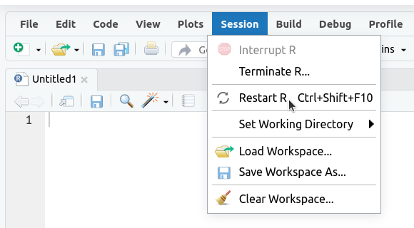
2. If the
Environmenttab isn’t empty click on the broom icon to clear it: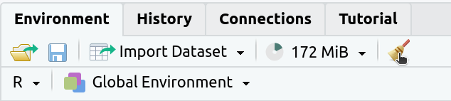
The
Environmenttab should now say “Environment Is Empty”: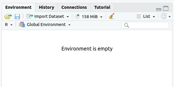
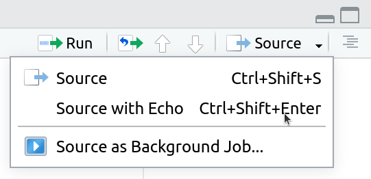
3. Rerun your entire homework assignment using “Source with Echo” to make sure it runs from start to finish and produces the expected results.
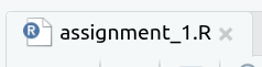
4. Make sure that you saved your code with the name
assignmentsomewhere in the file name. You should see the file in theFilestab and the name of the file should be black (not red with an*in the tab at the top of the text editor):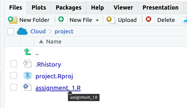
5. Make sure that your code will run on other computers
- No
setwd()(use RStudio Projects instead) - Use
/not\for paths
- No