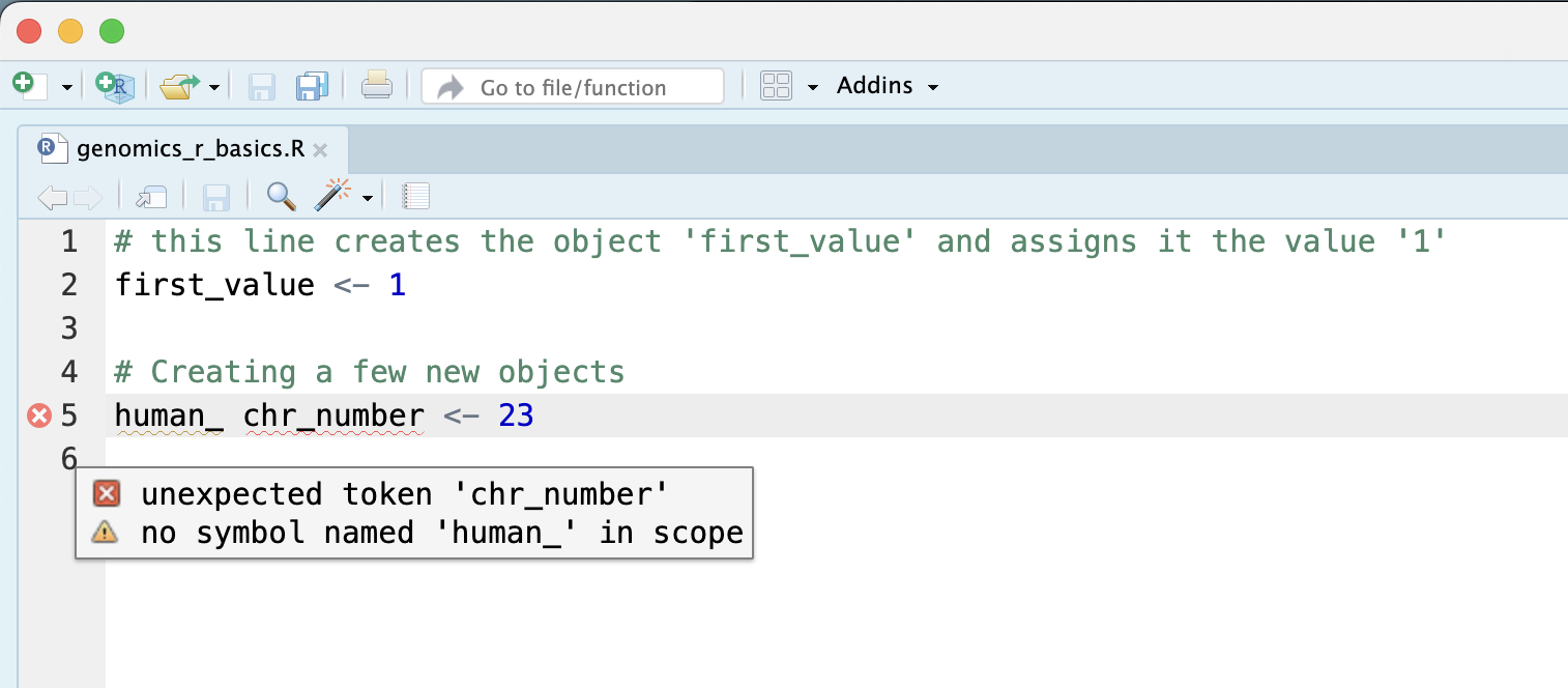
Image 1 of 1: ‘RStudio script editor where line 5, human_ chr_number <- 23, is marked with a red error icon and a tooltip reading unexpected token chr_number and no symbol named human_ in scope.’
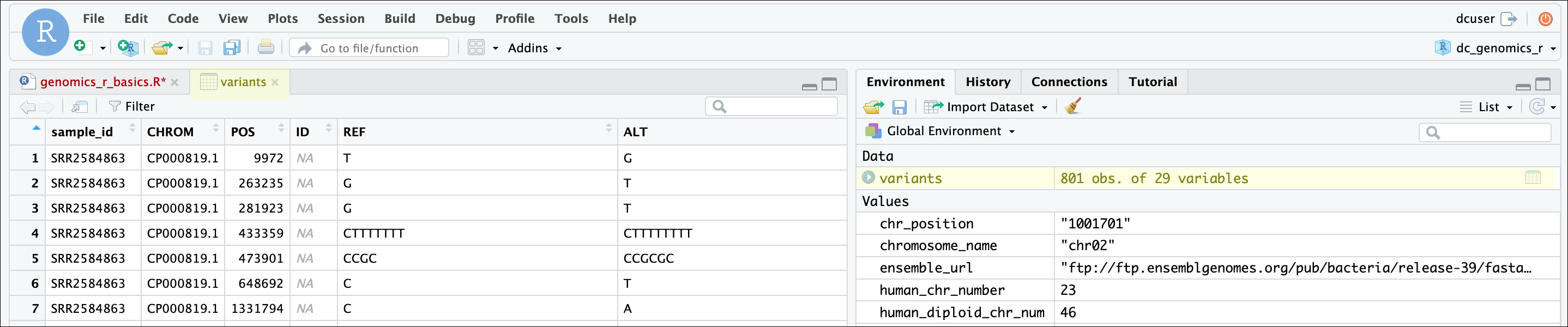
Image 1 of 1: ‘RStudio with the variants data frame open in a spreadsheet-style viewer tab showing columns such as sample_id, CHROM, POS, ID, REF and ALT, and the Environment pane listing variants as 801 obs. of 29 variables.’
RStudio data frame view
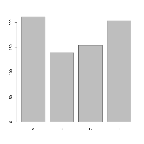
Figure 2
Image 1 of 1: ‘Bar plot of the number of SNPs for each alternative nucleotide, with bars for A, C, G and T in alphabetical order.’
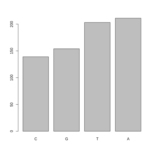
Figure 3
Image 1 of 1: ‘Bar plot of the number of SNPs for each alternative nucleotide, with the bars reordered from the least to the most frequent nucleotide.’
Figure 4
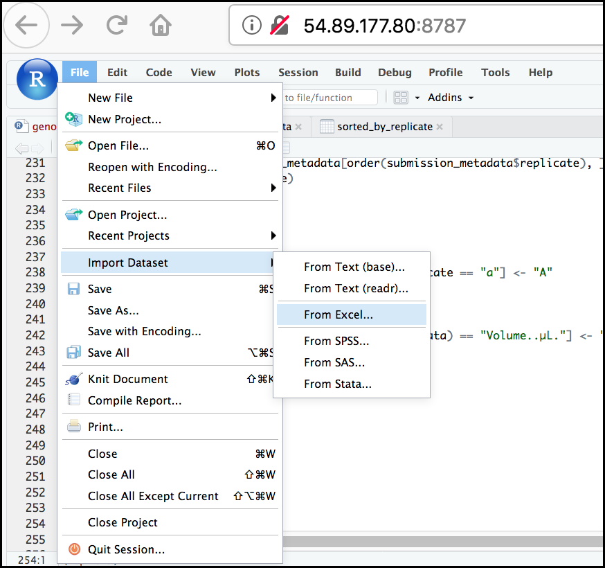
Image 1 of 1: ‘RStudio File menu opened with Import Dataset highlighted and its submenu showing From Excel... selected among options such as From Text (base), From Text (readr), From SPSS, From SAS and From Stata.’
RStudio import menu
Figure 5
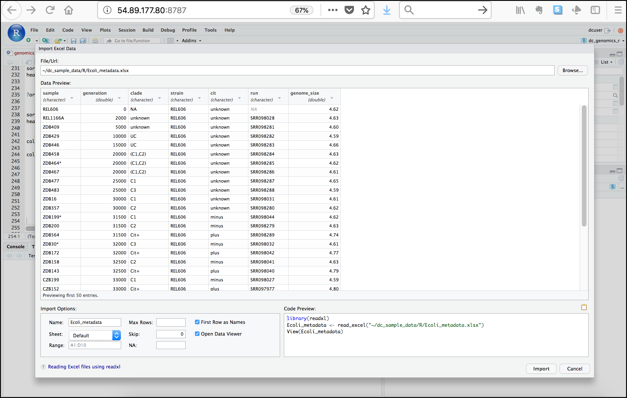
Image 1 of 1: ‘RStudio Import Excel Data dialog with the path to Ecoli_metadata.xlsx in the File/Url box, a data preview table with columns sample, generation, clade, strain, cit, run and genome_size, import options such as Name and Sheet, and a code preview using read_excel().’
Image 1 of 1: ‘Line plot enclosed in hexagon shape with ggplot2 typed beneath and www.rstudio.com at the bottom.’
Figure 2
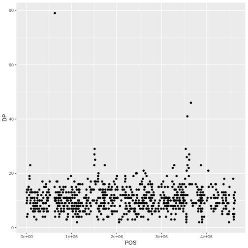
Image 1 of 1: ‘Scatter plot of read depth (DP) on the y-axis against base pair position (POS) on the x-axis, with one black point per variant.’
Figure 3
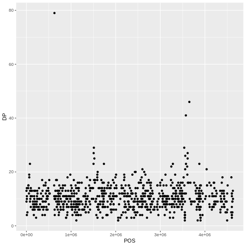
Image 1 of 1: ‘Scatter plot of read depth (DP) against base pair position (POS), with opaque black points that overlap in dense regions.’
Figure 4
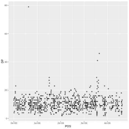
Image 1 of 1: ‘Scatter plot of read depth (DP) against base pair position (POS), now with semi-transparent points so overlapping points show up darker.’
Figure 5
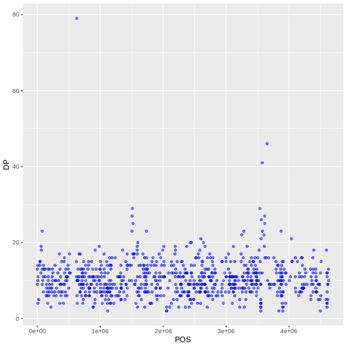
Image 1 of 1: ‘Scatter plot of read depth (DP) against base pair position (POS), with all points semi-transparent and colored blue.’
Figure 6
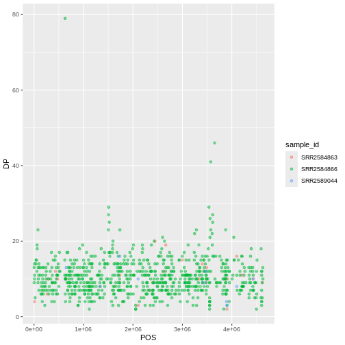
Image 1 of 1: ‘Scatter plot of read depth (DP) against base pair position (POS), with points colored by sample_id and a legend showing the three samples.’
Figure 7
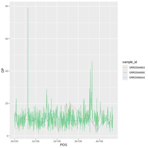
Image 1 of 1: ‘Line plot of read depth (DP) against base pair position (POS), with one semi-transparent line per sample colored by sample_id.’
Figure 8
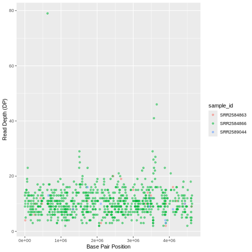
Image 1 of 1: ‘Scatter plot of read depth against base pair position, with points colored by sample_id and axes labelled Base Pair Position and Read Depth (DP).’
Figure 9
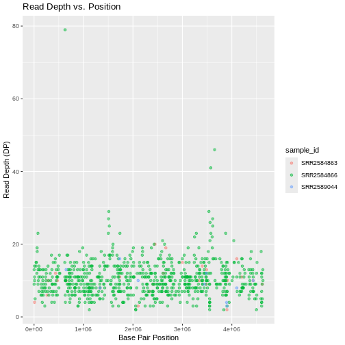
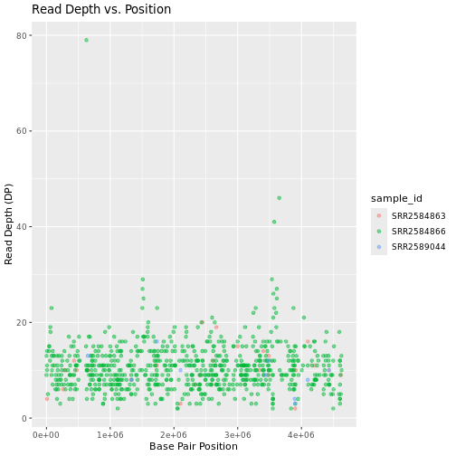
Image 1 of 1: ‘Scatter plot of read depth against base pair position, with points colored by sample_id, labelled axes and the title Read Depth vs. Position.’
Figure 10
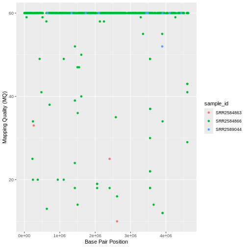
Image 1 of 1: ‘Scatter plot of mapping quality (MQ) against base pair position, with points colored by sample_id and axes labelled Base Pair Position and Mapping Quality (MQ).’
Figure 11
Image 1 of 1: ‘Scatter plot of read depth against base pair position, colored by sample_id, with title Read Depth vs. Position and all text in the Bookman font.’
Figure 12
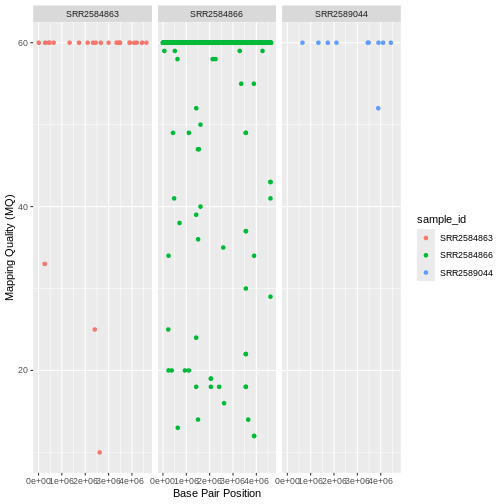
Image 1 of 1: ‘Scatter plot of mapping quality (MQ) against base pair position, split into three side-by-side panels, one per sample, with points colored by sample_id.’
Figure 13
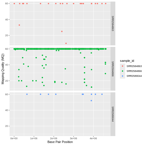
Image 1 of 1: ‘Scatter plot of mapping quality (MQ) against base pair position, split into three panels stacked vertically, one per sample, with points colored by sample_id.’
Figure 14
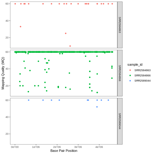
Image 1 of 1: ‘Scatter plot of mapping quality (MQ) against base pair position in three vertically stacked panels, one per sample, on a white background with no grid lines.’
Figure 15
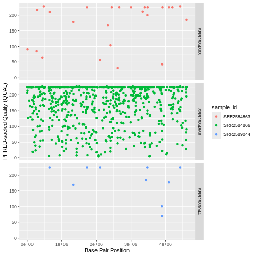
Image 1 of 1: ‘Scatter plot of PHRED-scaled quality (QUAL) against base pair position in three vertically stacked panels, one per sample, with points colored by sample_id.’
Figure 16
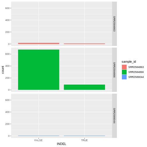
Image 1 of 1: ‘Bar plot of the number of variants that are indels (TRUE) or not (FALSE), in three vertically stacked panels, one per sample, with bars filled by sample_id and a legend.’
Figure 17
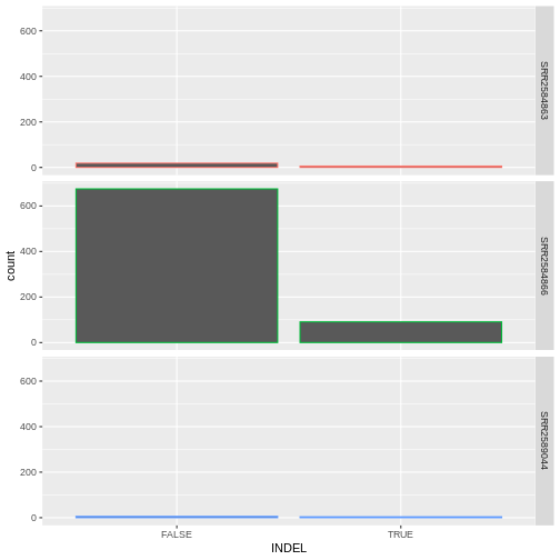
Image 1 of 1: ‘Bar plot of the number of variants that are indels (TRUE) or not (FALSE), in three vertically stacked panels, one per sample, with bar outlines colored by sample and no legend.’
Figure 18
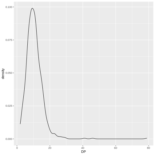
Image 1 of 1: ‘Density plot of read depth (DP), showing a single curve whose peak lies at about 10 reads.’
Figure 19
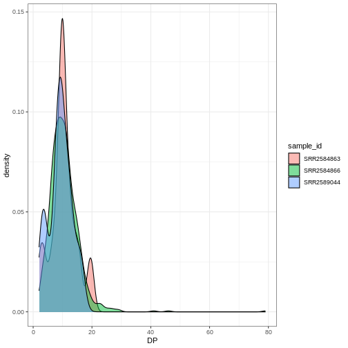
Image 1 of 1: ‘Density plot of read depth (DP) with one semi-transparent filled curve per sample, overlapping on a white background.’