Creating tables and views

Overview

Questions

• What is the difference between a table and a view?
• How can I create a table using the DB Browser for SQLite?
• How can I create a table or view in DB Browser for SQLite using SQL code?
• How can I add records of data to a table?

Objectives

• Understand the differences and similarities between Tables and Views
• Create table schemas using DB Browser for SQLite
• Create table schemas and views using SQL code
• Populate a table using SQL code
• Populate a table from a file of data using DB Browser for SQLite

Using SQL code to create tables

---

In relational databases, tables have to be created before you can add data to them. The table definition that you create is referred to as the Schema of the table.

The schema can contain many different properties of the table and the data that it does/will contain. In its simplest form you only need to specify a name for the table and a list of the column names and the data types for each of those columns.

In this episode we will also show how the Farms, Plots and Crops tables were created and populated from csv files. When we do this using DB Browser, it appears to be a single step process, much like importing a file into Excel. In fact it is always a two step process. First……………

Using the DB Browser application to create tables

---

So far we have created and populated tables from scratch or created tables from existing tables. But initially your data is likely to be external to the relational database system in a set of simple files. Typically in CSV (comma separated values) or Tab delimited format.

All relational database systems will have some utility which will allow you to import such files into tables in the database. The DB Browser application has a nice GUI (Graphical Use Interface) to allow you to do this.

The Farms, Plots and Crops tables that we have been using were created in the DB Browser application by importing a CSV file containing the data.

For large datasets this is a very common approach.

1. From the File menu select ‘Import’ and then ‘Table from CSV file’. This will start the ‘Import CSV file’ wizard and you will be asked to select the file of data you wish to import from a standard Windows file open dialog.

2. After you have selected the file, you will be shown the ‘Import CSV file’ window which will allow you to set a name for the table (the default is taken from the filename). You will see the first few rows of the data and there are a few options which can be changed if needs be.

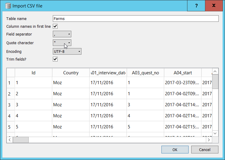
In our case all of the options are correctly set. If your file was in Tab delimited format, you would need to change the ‘Field separator’ option to ‘Tab’. If your file did not have a header row with column names you would un-check the appropriate box and DB Browser will allocate names for the columns. (You can change them to more meaningful names yourself after the import is complete)

3. When you click OK, a table will be created and the data loaded into the table.

Unfortunately this Import wizard in DB Browser does not do, or allow you to do everything that you might want when creating a table. The most obvious potential problem is that we were not allowed to specify the data types to be associated with each of the columns in the table. However, DB Browser will attempt to work out the appropriate data types based on the values in the first few rows of the data. This is a very common approach. (Earlier versions of DB Browser didn’t do this, it just imported all of the columns as ‘Text’ data types.) If you go to the table in the Database Structure tab and click the ‘>’ you will see all of the fields and they are all listed as either Text or Integer fields.

If any of the datatypes are not as expected or wanted we can change them.

4. Select the newly created table in Database Structure tab and click the ‘Modify Table’ button in the toolbar. The ‘Edit Table Definition’ dialog will appear.

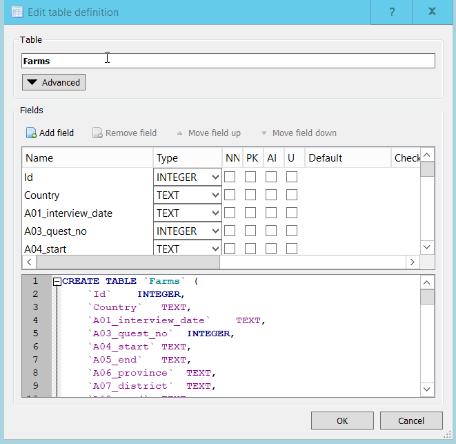
In this particular case DB Browser correctly selected the datatypes. Notice that the A01_interview_date was allocated a datatype of ‘TEXT’. This isn’t a problem as we have to use the Date and Time functions to manipulate dates anyway.

Notice that the bottom pane in the Window shows the SQL DDL statement that would create the table that you modifying.

When you change one of the columns from TEXT to INTEGER, this is immediately reflected in the Create Table statement.
It is slightly misleading because in fact we are modifying an existing table and in SQL-speak, this would be an Alter Table… statement. However it does illustrate quite well the fact that whatever you do in the GUI, it is essentially translated into an SQL statement and executed. You could copy and paste this definition into the SQL editor and if you change the table name before you ran it, you would create a new table with that name. This new table would have no data in it. This is how the insert table wizard works. It uses the header row from your data to create a CREATE TABLE statement which it runs. It then transforms each of the rows of data into SQL INSERT INTO... statements which it also runs to get the data into the table.

In addition to changing the data types there are several other options which can be set when you are creating of modifying a table. For our tables we don’t need to make use of them but for completeness we will describe what they are;

PK - Or Primary Key, a unique identifier for the row. In the Farms table, there is an Id column which uniquely identifies a Farm. This could act as a unique identifier for the row as a whole. We could mark this as the primary key if we wanted to.

AI - Or Auto Increment. This isn’t really applicable to tables created in this way, i.e. the creation of the schema immediately followed by loading data from a file. It is usually used to generate unique values for a column which could then act as a primary key. If you have an ‘Auto Increment’ column in a table, when you insert values you would not supply a value for the column as SQLite will automatically provide a value for each row added.

Not Null - If this is checked then it means that there must be a value for each row in this column. If it is not set and there is no value provided in the data then it will be set to ‘NULL’ which means ‘I know nothing about what should be here’. (Not the string ‘NULL’ but the NULL value)

In real datasets missing values are quite common and we have already looked at ways of dealing with them when they occur in tables. If you were to check this box and the data did have missing values for this column, the record from the file would be rejected and the load of the file will fail.

U - Or Unique. This allows you to say that the contents of the column, which is not the primary key column has to have unique values in it. Like Allow Null this is another way of providing some data validation as the data is imported. Although it doesn’t really apply with the DB Browser import wizard as the data is imported before you are allowed to set this option.

Default - This is used in conjunction with ‘Not Null’, if a value is not provided in the dataset, then if provided, the default value for that column will be used.

Check - This allows you to specify a constraint on the values entered for the column. You could restrict the range of values or compare the value with other columns values.

These three options, ‘Not Null’, ‘Unique’ and ‘Default’ , need to be used with caution and certainly their use needs to be fully documented and explained.

Exercise

From the Modify table dialog, change the Id column in the Farms table to be the primary key. What difference did it make in the CREATE TABLE statement?

Show me the solution

You need to scroll down to the bottom of the CREATE TABLE statement to see the

SQL

    PRIMARY KEY(`Id`)

line added.

Creating a table using an SQL command

---

You could copy and paste this definition into the SQL editor and if you change the table name before you ran it, you would create a new table with that name. This new table would have no data in it. This is how the insert table wizard works. It uses the header row from your data to create a CREATE TABLE statement which it runs. It then transforms each of the rows of data into SQL INSERT INTO... statements which it also runs to get the data into the table.

For small tables defining them and populating them with data in this way may be acceptable. But for larger tables this approach not only to defining the tables but adding potentially thousands of rows of data can be somewhat impractical.

Creating tables from other tables

---

Whenever you write a Select query and run it, the results are always in the form of a table. In the results pane, you can see the column names and the rows of data in the results.

This provides a very easy way of creating a new table based on the results of a query.

The following query selects a few of the columns from the Farms table:

SQL

SELECT Id, 
       Country, 
       A06_province, 
       A07_district,
       A08_ward, 
       A09_village
FROM Farms;

If you want to make the results of this query into a new table, you can do so by simply prefixing the SELECT with CREATE TABLE NewTablename AS like this:

SQL

CREATE TABLE Farms_location AS
SELECT Id, 
       Country, 
       A06_province, 
       A07_district,
       A08_ward, 
       A09_village
FROM Farms;

If we wanted to create a table from the Crops table which contains only the rows where the D_curr_crop value was ‘rice’ we could use a query like this:

SQL

CREATE TABLE crops_rice AS
SELECT *
FROM Crops
WHERE D_curr_crop = 'rice'
;

Here we want all of the columns from the Crops table but only if the D_curr_crop value is ‘rice’.

Note: please ensure that you run the code above as we will use this new table in a later episode.

Using SQL code to create views

---

In addition to tables all relational database systems have the concept of ‘Views’. Views are based on tables. In the same way that we were able to create a table based on a SELECT query, we can create a ‘View’ in the same way. You just replace ‘Table’ with ‘View’.

SQL

CREATE VIEW Farms_location AS
SELECT Id, 
       Country, 
       A06_province, 
       A07_district,
       A08_ward, 
       A09_village
FROM Farms;

Tables and Views are so closely related that if you try to run the code above, although ‘Table’ has been changed to ‘View’ you will get an error complaining that the ‘Table’ already exists.

It is common practice when creating Views to indicate somewhere in the name that it is in fact a View. e.g. vFarms_location or Farms_location_v.

Although tables and views can be used almost interchangeably in SELECT queries it is important to note that a View unlike a Table contains no data. It is essentially the SQL statement needed to produce that data from the underlying data. This means that when you use a View there is the overhead of having to run this SQL first. Although in practice the Database system will combine the SQL required by the View and the other SQL in your query so as to optimise how the SQL is executed.

The advantage of using Views is that it allows you to restrict how you see the data in a table. In the example we used above it may be far easier to work with only the 6 columns that we need from the full Farms table rather than the full table with 61 columns.

A View isn’t restricted to simple SELECT statements it can be the result of aggregations and joins as well. This can help reduce the complexity of queries based on the View and so aid readability.

Key Points

• Database tables can be created using the DDL command CREATE TABLE
• They can be populated using the INSERT INTO command
• The SQLite plugin allows you to create a table and import data into it in one step
• There are many options available to the CREATE TABLE command which allows greater control over how or what data can be loaded into the table
• A View can be treated just like a table in a query
• A View does not contain data like a table does, only the instructions on how to get the data