Basic Queries
Last updated on 2025-12-12 | Edit this page
Overview
Questions
- How can we select and download the data we want from the Gaia server?
Objectives
- Compose a basic query in ADQL/SQL.
- Use queries to explore a database and its tables.
- Use queries to download data.
- Develop, test, and debug a query incrementally.
As a running example, we will replicate parts of the analysis in the paper, “Off the beaten path: Gaia reveals GD-1 stars outside of the main stream” by Adrian Price-Whelan and Ana Bonaca.
Outline
This episode demonstrates the steps for selecting and downloading data from the Gaia Database:
First we will make a connection to the Gaia server,
We will explore information about the database and the tables it contains,
We will write a query and send it to the server, and finally
We will download the response from the server.
Query Language
In order to select data from a database, you need to compose a query, which is a program written in a “query language”. The query language we will use is ADQL, which stands for “Astronomical Data Query Language”.
ADQL is a dialect of SQL (Structured Query Language), which is by far the most commonly used query language. Almost everything you will learn about ADQL also works in SQL.
The reference manual for ADQL is here. But you might find it easier to learn from this ADQL Cookbook.
Using Jupyter
If you have not worked with Jupyter notebooks before, you might start with the tutorial from Jupyter.org called “Try Classic Notebook”, or this tutorial from DataQuest.
There are two environments you can use to write and run notebooks:
“Jupyter Notebook” is the original, and
“Jupyter Lab” is a newer environment with more features.
For this lesson, you can use either one.
Here are the most important things to know about running a Jupyter notebook:
Notebooks are made up of code cells and text cells (and a few other less common kinds). Code cells contain code; text cells contain explanatory text written in Markdown.
To run a code cell, click the cell to select it and press Shift-Enter. The output of the code should appear below the cell.
In general, notebooks only run correctly if you run every code cell in order from top to bottom. If you run cells out of order, you are likely to get errors.
You can modify existing cells, but then you have to run them again to see the effect.
You can add new cells, but you need to be careful about the order you run them in.
If you have added or modified cells, and the behavior of the notebook seems strange, you can restart the “kernel”, which clears all of the variables and functions you have defined, and run the cells again from the beginning.
If you are using Jupyter Notebook, open the
Kernelmenu and select “Restart and Run All”.In Jupyter Lab, open the
Kernelmenu and select “Restart Kernel and Run All Cells”.
Before you continue with this lesson, you might want to explore the other menus and the toolbar to see what else you can do.
Connecting to Gaia
The library we will use to get Gaia data is Astroquery.
Astroquery provides Gaia, which is an object
that represents a connection to the Gaia database.
We can connect to the Gaia database like this:
Old versions of astroquery output
if you are using a version of astroquery that’s older than v0.4.4, you may see this output
OUTPUT
Created TAP+ (v1.2.1) - Connection:
	Host: gea.esac.esa.int
	Use HTTPS: True
	Port: 443
	SSL Port: 443
Created TAP+ (v1.2.1) - Connection:
	Host: geadata.esac.esa.int
	Use HTTPS: True
	Port: 443
	SSL Port: 443
This import statement creates a TAP+ connection; TAP stands for “Table Access Protocol”, which is a network protocol for sending queries to the database and getting back the results.
Databases and Tables
What is a database? Most generally, it can be any collection of data, but when we are talking about ADQL or SQL:
A database is a collection of one or more named tables.
Each table is a 2-D array with one or more named columns of data.
We can use Gaia.load_tables to get the names of the
tables in the Gaia database. With the option
only_names=True, it loads information about the tables,
called “metadata”, but not the data itself.
OUTPUT
INFO: Retrieving tables... [astroquery.utils.tap.core]
INFO: Parsing tables... [astroquery.utils.tap.core]
INFO: Done. [astroquery.utils.tap.core]
The following for loop prints the names of the
tables.
OUTPUT
external.apassdr9
external.gaiadr2_geometric_distance
external.gaiaedr3_distance
external.galex_ais
external.ravedr5_com
external.ravedr5_dr5
external.ravedr5_gra
external.ravedr5_on
external.sdssdr13_photoprimary
external.skymapperdr1_master
external.skymapperdr2_master
[Output truncated]
So that is a lot of tables. The ones we will use are:
gaiadr2.gaia_source, which contains Gaia data from data release 2,gaiadr2.panstarrs1_original_valid, which contains the photometry data we will use from PanSTARRS, andgaiadr2.panstarrs1_best_neighbour, which we will use to cross-match each star observed by Gaia with the same star observed by PanSTARRS.
We can use load_table (not load_tables) to
get the metadata for a single table. The name of this function is
misleading, because it only downloads metadata, not the contents of the
table.
OUTPUT
Retrieving table 'gaiadr2.gaia_source'
Parsing table 'gaiadr2.gaia_source'...
Done.

<astroquery.utils.tap.model.taptable.TapTableMeta at 0x7f50edd2aeb0>
Jupyter shows that the result is an object of type
TapTableMeta, but it does not display the contents.
To see the metadata, we have to print the object.
OUTPUT
TAP Table name: gaiadr2.gaiadr2.gaia_source
Description: This table has an entry for every Gaia observed source as listed in the
Main Database accumulating catalogue version from which the catalogue
release has been generated. It contains the basic source parameters,
that is only final data (no epoch data) and no spectra (neither final
nor epoch).
Size (bytes): 4906520690688
Num. columns: 96
Columns
The following loop prints the names of the columns in the table.
OUTPUT
solution_id
designation
source_id
random_index
ref_epoch
ra
ra_error
dec
dec_error
parallax
parallax_error
[Output truncated]
You can probably infer what many of these columns are by looking at the names, but you should resist the temptation to guess. To find out what the columns mean, read the documentation.
Exercise (2 minutes)
One of the other tables we will use is
gaiadr2.panstarrs1_original_valid. Use
load_table to get the metadata for this table. How many
columns are there and what are their names?
PYTHON
panstarrs_metadata = Gaia.load_table('gaiadr2.panstarrs1_original_valid')
print(panstarrs_metadata)
OUTPUT
Retrieving table 'gaiadr2.panstarrs1_original_valid'
TAP Table name: gaiadr2.gaiadr2.panstarrs1_original_valid
Description: The Panoramic Survey Telescope and Rapid Response System (Pan-STARRS) is
a system for wide-field astronomical imaging developed and operated by
the Institute for Astronomy at the University of Hawaii. Pan-STARRS1

[Output truncated]

Catalogue curator:
SSDC - ASI Space Science Data Center
https://www.ssdc.asi.it/
Size (bytes): 933802426368
Num. columns: 26OUTPUT
obj_name
obj_id
ra
dec
ra_error
dec_error
epoch_mean
g_mean_psf_mag
g_mean_psf_mag_error
g_flags
r_mean_psf_mag
r_mean_psf_mag_error
r_flags
i_mean_psf_mag
i_mean_psf_mag_error
i_flags
z_mean_psf_mag
z_mean_psf_mag_error
z_flags
y_mean_psf_mag
y_mean_psf_mag_error
y_flags
n_detections
zone_id
obj_info_flag
quality_flag
Writing queries
You might be wondering how we download these tables. With tables this big, you generally don’t. Instead, you use queries to select only the data you want.
A query is a program written in a query language like SQL. For the Gaia database, the query language is a dialect of SQL called ADQL.
Here’s an example of an ADQL query.
Triple-quotes strings
We use a triple-quoted string here so we can include line breaks in the query, which makes it easier to read.
The words in uppercase are ADQL keywords:
SELECTindicates that we are selecting data (as opposed to adding or modifying data).TOPindicates that we only want the first 10 rows of the table, which is useful for testing a query before asking for all of the data.FROMspecifies which table we want data from.
The third line is a list of column names, indicating which columns we want.
In this example, the keywords are capitalized and the column names are lowercase. This is a common style, but it is not required. ADQL and SQL are not case-sensitive.
Also, the query is broken into multiple lines to make it more readable. This is a common style, but not required. Line breaks don’t affect the behavior of the query.
To run this query, we use the Gaia object, which
represents our connection to the Gaia database, and invoke
launch_job:
OUTPUT
<astroquery.utils.tap.model.job.Job at 0x7f50edd2adc0>The result is an object that represents the job running on a Gaia server.
If you print it, it displays metadata for the forthcoming results.
OUTPUT
<Table length=10>
   name    dtype  unit                            description                             n_bad
--------- ------- ---- ------------------------------------------------------------------ -----
source_id   int64      Unique source identifier (unique within a particular Data Release)     0
       ra float64  deg                                                    Right ascension     0
      dec float64  deg                                                        Declination     0
 parallax float64  mas                                                           Parallax     2
Jobid: None
Phase: COMPLETED
Owner: None
Output file: sync_20210315090602.xml.gz
[Output truncated]
Don’t worry about Results: None. That does not actually
mean there are no results.
However, Phase: COMPLETED indicates that the job is
complete, so we can get the results like this:
OUTPUT
astropy.table.table.TableThe type function indicates that the result is an Astropy Table.
Repetition
Why is table repeated three times? The first is the name
of the module, the second is the name of the submodule, and the third is
the name of the class. Most of the time we only care about the last one.
It’s like the Linnean name for the Western lowland gorilla, which is
Gorilla gorilla gorilla.
An Astropy Table is similar to a table in an SQL
database except:
SQL databases are stored on disk drives, so they are persistent; that is, they “survive” even if you turn off the computer. An Astropy
Tableis stored in memory; it disappears when you turn off the computer (or shut down your Jupyter notebook).SQL databases are designed to process queries. An Astropy
Tablecan perform some query-like operations, like selecting columns and rows. But these operations use Python syntax, not SQL.
Jupyter knows how to display the contents of a
Table.
OUTPUT
<Table length=10>
     source_id              ra                 dec               parallax
                           deg                 deg                 mas
       int64             float64             float64             float64
------------------- ------------------ ------------------- --------------------
5887983246081387776   227.978818386372  -53.64996962450103   1.0493172163332998
5887971250213117952 228.32280834041364  -53.66270726203726  0.29455652682279093
5887991866047288704  228.1582047014091 -53.454724911639794  -0.5789179941669236
5887968673232040832 228.07420888099884   -53.8064612895961  0.41030970779603076
5887979844465854720 228.42547805195946  -53.48882284470035 -0.23379683441525864
5887978607515442688 228.23831627636855  -53.56328249482688  -0.9252161956789068
[Output truncated]
Each column has a name, units, and a data type.
For example, the units of ra and dec are
degrees, and their data type is float64, which is a 64-bit
floating-point
number, used to store measurements with a fraction part.
This information comes from the Gaia database, and has been stored in
the Astropy Table by Astroquery.
Exercise (3 minutes)
Read the documentation of this table and choose a column that looks interesting to you. Add the column name to the query and run it again. What are the units of the column you selected? What is its data type?
For example, we can add radial_velocity : Radial velocity (double, Velocity[km/s] ) - Spectroscopic radial velocity in the solar barycentric reference frame. The radial velocity provided is the median value of the radial velocity measurements at all epochs.
PYTHON
query1_with_rv = """SELECT
TOP 10
source_id, ra, dec, parallax, radial_velocity
FROM gaiadr2.gaia_source
"""
job1_with_rv = Gaia.launch_job(query1_with_rv)
results1_with_rv = job1_with_rv.get_results()
results1_with_rv
OUTPUT
     source_id              ra         ...       parallax       radial_velocity
                           deg         ...         mas               km / s
------------------- ------------------ ... -------------------- ---------------
5800603716991968256 225.13905251174302 ...   0.5419737483675161              --
5800592790577127552 224.30113911598448 ...  -0.6369101209622813              --
5800601273129497856 225.03260084885449 ...  0.27554460953986526              --
[Output truncated]
Asynchronous queries
launch_job asks the server to run the job
“synchronously”, which normally means it runs immediately. But
synchronous jobs are limited to 2000 rows. For queries that return more
rows, you should run “asynchronously”, which mean they might take longer
to get started.
If you are not sure how many rows a query will return, you can use
the SQL command COUNT to find out how many rows are in the
result without actually returning them. We will see an example in the
next lesson.
The results of an asynchronous query are stored in a file on the server, so you can start a query and come back later to get the results. For anonymous users, files are kept for three days.
As an example, let us try a query that is similar to
query1, with these changes:
It selects the first 3000 rows, so it is bigger than we should run synchronously.
It selects two additional columns,
pmraandpmdec, which are proper motions along the axes ofraanddec.It uses a new keyword,
WHERE.
PYTHON
query2 = """SELECT
TOP 3000
source_id, ra, dec, pmra, pmdec, parallax
FROM gaiadr2.gaia_source
WHERE parallax < 1
"""
A WHERE clause indicates which rows we want; in this
case, the query selects only rows “where” parallax is less
than 1. This has the effect of selecting stars with relatively low
parallax, which are farther away. We’ll use this clause to exclude
nearby stars that are unlikely to be part of GD-1.
WHERE is one of the most common clauses in ADQL/SQL, and
one of the most useful, because it allows us to download only the rows
we need from the database.
We use launch_job_async to submit an asynchronous
query.
OUTPUT
INFO: Query finished. [astroquery.utils.tap.core]

<astroquery.utils.tap.model.job.Job at 0x7f50edd40f40>
And here are the results.
OUTPUT
<Table length=3000>
     source_id              ra         ...       parallax       radial_velocity
                           deg         ...         mas               km / s
       int64             float64       ...       float64            float64
------------------- ------------------ ... -------------------- ---------------
5895270396817359872 213.08433715252883 ...    2.041947005434917              --
5895272561481374080  213.2606587905109 ...  0.15693467895110133              --
5895247410183786368 213.38479712976664 ... -0.19017525742552605              --
5895249226912448000 213.41587389088238 ...                   --              --
5895261875598904576  213.5508930114549 ... -0.29471722363529257              --
5895258302187834624 213.87631129557286 ...   0.6468437015289753              --
[Output truncated]
You might notice that some values of parallax are
negative. As this
FAQ explains, “Negative parallaxes are caused by errors in the
observations.” They have “no physical meaning,” but they can be a
“useful diagnostic on the quality of the astrometric solution.”
Different results
Your results for this query may differ from the Instructor’s. This is
because TOP 3000 returns 3000 results, but those results
are not organized in any particular way.
Exercise (5 minutes)
The clauses in a query have to be in the right order. Go back and
change the order of the clauses in query2 and run it again.
The modified query should fail, but notice that you don’t get much
useful debugging information.
For this reason, developing and debugging ADQL queries can be really hard. A few suggestions that might help:
Whenever possible, start with a working query, either an example you find online or a query you have used in the past.
Make small changes and test each change before you continue.
While you are debugging, use
TOPto limit the number of rows in the result. That will make each test run faster, which reduces your development time.Launching test queries synchronously might make them start faster, too.
In this example, the WHERE clause is in the wrong place.
ERROR
query2_erroneous = """SELECT
TOP 3000
source_id, ra, dec, pmra, pmdec, parallax
FROM gaiadr2.gaia_source
WHERE parallax < 1
"""
Operators
In a WHERE clause, you can use any of the SQL comparison
operators; here are the most common ones:
| Symbol | Operation |
|---|---|
> |
greater than |
< |
less than |
>= |
greater than or equal |
<= |
less than or equal |
= |
equal |
!= or <>
|
not equal |
Most of these are the same as Python, but some are not. In
particular, notice that the equality operator is =, not
==. Be careful to keep your Python out of your ADQL!
You can combine comparisons using the logical operators:
- AND: true if both comparisons are true
- OR: true if either or both comparisons are true
Finally, you can use NOT to invert the result of a
comparison.
Exercise (5 minutes)
Read about
SQL operators here and then modify the previous query to select rows
where bp_rp is between -0.75 and
2.
bp_rp contains BP-RP color, which is the difference
between two other columns, phot_bp_mean_mag and
phot_rp_mean_mag. You can read
about this variable here.
This Hertzsprung-Russell diagram shows the BP-RP color and luminosity of stars in the Gaia catalog (Copyright: ESA/Gaia/DPAC, CC BY-SA 3.0 IGO).
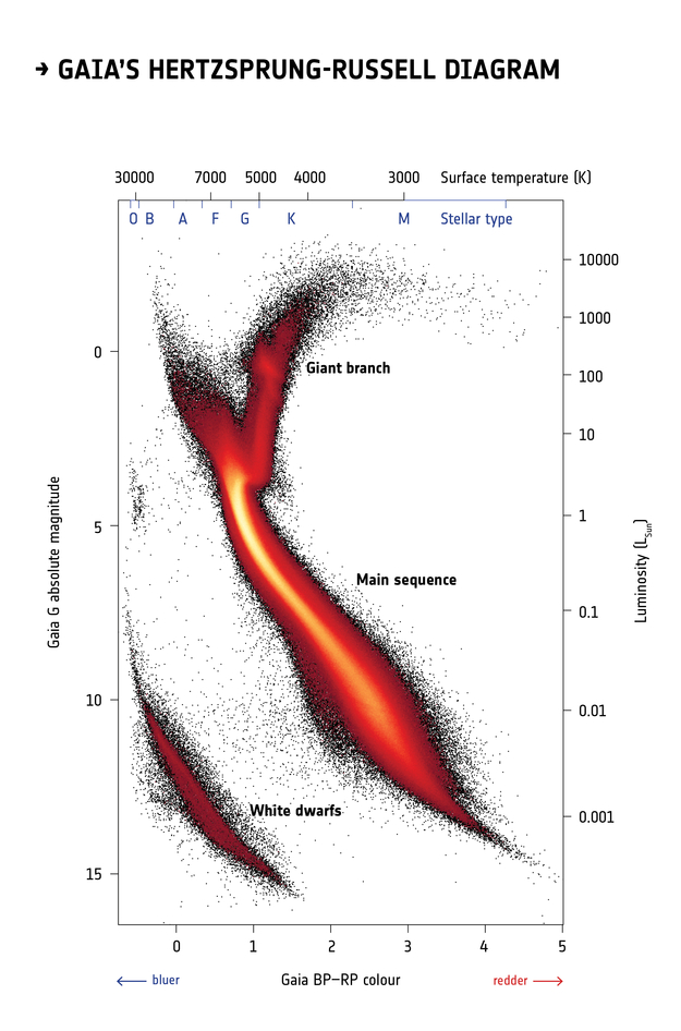
Selecting stars with bp-rp less than 2 excludes many class M dwarf stars, which are low
temperature, low luminosity. A star like that at GD-1’s distance would
be hard to detect, so if it is detected, it is more likely to be in the
foreground.
Formatting queries
The queries we have written so far are string “literals”, meaning that the entire string is part of the program. But writing queries yourself can be slow, repetitive, and error-prone.
It is often better to write Python code that assembles a query for
you. One useful tool for that is the string
format method.
As an example, we will divide the previous query into two parts; a list of column names and a “base” for the query that contains everything except the column names.
Here is the list of columns we will select.
And here is the base. It is a string that contains at least one format specifier in curly brackets (braces).
PYTHON
query3_base = """SELECT
TOP 10
{columns}
FROM gaiadr2.gaia_source
WHERE parallax < 1
  AND bp_rp BETWEEN -0.75 AND 2
"""
This base query contains one format specifier,
{columns}, which is a placeholder for the list of column
names we will provide.
To assemble the query, we invoke format on the base
string and provide a keyword argument that assigns a value to
columns.
In this example, the variable that contains the column names and the variable in the format specifier have the same name. That is not required, but it is a common style.
The result is a string with line breaks. If you display it, the line
breaks appear as \n.
OUTPUT
'SELECT \nTOP 10 \nsource_id, ra, dec, pmra, pmdec, parallax\nFROM gaiadr2.gaia_source\nWHERE parallax < 1\n AND bp_rp BETWEEN -0.75 AND 2\n'But if you print it, the line breaks appear as line breaks.
OUTPUT
SELECT
TOP 10
source_id, ra, dec, pmra, pmdec, parallax
FROM gaiadr2.gaia_source
WHERE parallax < 1
  AND bp_rp BETWEEN -0.75 AND 2
Notice that the format specifier has been replaced with the value of
columns.
Let’s run it and see if it works:
OUTPUT
<Table length=10>
   name    dtype    unit                              description
--------- ------- -------- ------------------------------------------------------------------
source_id   int64          Unique source identifier (unique within a particular Data Release)
       ra float64      deg                                                    Right ascension
      dec float64      deg                                                        Declination
     pmra float64 mas / yr                         Proper motion in right ascension direction
    pmdec float64 mas / yr                             Proper motion in declination direction
 parallax float64      mas                                                           Parallax
Jobid: None
Phase: COMPLETED
Owner: None
[Output truncated]OUTPUT
<Table length=10>
     source_id              ra         ...       parallax
                           deg         ...         mas
------------------- ------------------ ... -------------------
3031147124474711552 110.10540720349103 ... 0.47255775887968876
3031114276567648256 110.92831846731636 ... 0.41817219481822415
3031130872315906048 110.61072654450903 ...   0.178490206751036
3031128162192428544 110.78664993513391 ...  0.8412331482786942
3031140497346996736  110.0617759777779 ... 0.16993569795437397
3031111910043832576 110.84459425332385 ...  0.4668864606089576
[Output truncated]Exercise (10 minutes)
This query always selects sources with parallax less
than 1. But suppose you want to take that upper bound as an input.
Modify query3_base to replace 1 with a
format specifier like {max_parallax}. Now, when you call
format, add a keyword argument that assigns a value to
max_parallax, and confirm that the format specifier gets
replaced with the value you provide.
Summary
This episode has demonstrated the following steps:
Making a connection to the Gaia server,
Exploring information about the database and the tables it contains,
Writing a query and sending it to the server, and finally
Downloading the response from the server as an Astropy
Table.
In the next episode we will extend these queries to select a particular region of the sky.
- If you can’t download an entire dataset (or it is not practical) use queries to select the data you need.
- Read the metadata and the documentation to make sure you understand the tables, their columns, and what they mean.
- Develop queries incrementally: start with something simple, test it, and add a little bit at a time.
- Use ADQL features like
TOPandCOUNTto test before you run a query that might return a lot of data. - If you know your query will return fewer than 3000 rows, you can run it synchronously. If it might return more than 3000 rows, you should run it asynchronously.
- ADQL and SQL are not case-sensitive. You don’t have to capitalize the keywords, but it will make your code more readable.
- ADQL and SQL don’t require you to break a query into multiple lines, but it will make your code more readable.
- Make each section of the notebook self-contained. Try not to use the same variable name in more than one section.
- Keep notebooks short. Look for places where you can break your analysis into phases with one notebook per phase.