Plotting and Tabular Data
Last updated on 2026-06-19 | Edit this page
Overview
Questions
- How do we make scatter plots in Matplotlib?
- How do we store data in a pandas
DataFrame?
Objectives
- Select rows and columns from an Astropy
Table. - Use Matplotlib to make a scatter plot.
- Use Gala to transform coordinates.
- Make a pandas
DataFrameand use a BooleanSeriesto select rows. - Save a
DataFramein an HDF5 file.
In the previous episode, we wrote a query to select stars from the region of the sky where we expect GD-1 to be, and saved the results in a FITS file.
Now we will read that data back in and implement the next step in the analysis, identifying stars with the proper motion we expect for GD-1.
Outline
We will read back the results from the previous lesson, which we saved in a FITS file.
Then we will transform the coordinates and proper motion data from ICRS back to the coordinate frame of GD-1.
We will put those results into a pandas
DataFrame.
Starting from this episode
If you are starting a new notebook for this episode, expand this section for information you will need to get started.
In the previous episode, we ran a query on the Gaia server, downloaded data for roughly 140,000 stars, and saved the data in a FITS file. We will use that data for this episode. Whether you are working from a new notebook or coming back from a checkpoint, reloading the data will save you from having to run the query again.
If you are starting this episode here or starting this episode in a
new notebook, you will need to run the following lines of code. The last
two lines of the import statements assume your notebook is being run in
the student_download directory. If you are running it from
a different directory you will need to add the path using
sys.path.append(<path to student download>) where
<path to student_download> is the path to your
student_download directory ending with
student_download.
This imports previously imported functions:
PYTHON
import astropy.units as u
from astropy.coordinates import SkyCoord
from astropy.table import Table

from episode_functions import *
from gd1 import GD1Koposov10
The following code loads in the data (instructions for downloading
data can be found in the setup instructions).
You may need to add a the path to the filename variable below
(e.g. filename = 'student_download/backup-data/gd1_results.fits')
Selecting rows and columns
In the previous episode, we selected spatial and proper motion
information from the Gaia catalog for stars around a small part of GD-1.
The output was returned as an Astropy Table. We can use
info to check the contents.
OUTPUT
<Table length=140339>
   name    dtype    unit                              description
--------- ------- -------- ------------------------------------------------------------------
source_id   int64          Unique source identifier (unique within a particular Data Release)
       ra float64      deg                                                    Right ascension
      dec float64      deg                                                        Declination
     pmra float64 mas / yr                         Proper motion in right ascension direction
    pmdec float64 mas / yr                             Proper motion in declination direction
 parallax float64      mas                                                           Parallax
In this episode, we will see operations for selecting columns and
rows from an Astropy Table. You can find more information
about these operations in the Astropy
documentation.
We can get the names of the columns like this:
OUTPUT
['source_id', 'ra', 'dec', 'pmra', 'pmdec', 'parallax']And select an individual column like this:
OUTPUT
<Column name='ra' dtype='float64' unit='deg' description='Right ascension' length=140339>
142.48301935991023
142.25452941346344
142.64528557468074
142.57739430926034
142.58913564478618
141.81762228999614
143.18339801317677
 142.9347319464589
142.26769745823267
142.89551292869012
[Output truncated]
The result is a Column object that contains the data,
and also the data type, units, and name of the column.
OUTPUT
astropy.table.column.ColumnThe rows in the Table are numbered from 0 to
n-1, where n is the number of rows. We can
select the first row like this:
OUTPUT
<Row index=0>
    source_id              ra                dec                pmra              pmdec             parallax
                          deg                deg              mas / yr           mas / yr             mas
      int64             float64            float64            float64            float64            float64
------------------ ------------------ ----------------- ------------------- ----------------- -------------------
637987125186749568 142.48301935991023 21.75771616932985 -2.5168384683875766 2.941813096629439 -0.2573448962333354
The result is a Row object.
OUTPUT
astropy.table.row.RowNotice that the bracket operator can be used to select both columns and rows. You might wonder how it knows which to select. If the expression in brackets is a string, it selects a column; if the expression is an integer, it selects a row.
If you apply the bracket operator twice, you can select a column and then an element from the column.
OUTPUT
np.float64(142.48301935991023)Or you can select a row and then an element from the row.
OUTPUT
np.float64(142.48301935991023)You get the same result either way.
Scatter plot
To see what the results look like, we will use a scatter plot. The library we will use is Matplotlib, which is the most widely-used plotting library for Python. The Matplotlib interface is based on MATLAB (hence the name), so if you know MATLAB, some of it will be familiar.
We will import like this:
Pyplot is part of the Matplotlib library. It is conventional to
import it using the shortened name plt.
Keeping plots in the notebook
In recent versions of Jupyter, plots appear “inline”; that is, they are part of the notebook. In some older versions, plots appear in a new window. If your plots appear in a new window, you might want to run the following Jupyter magic command in a notebook cell:
Pyplot provides two functions that can make scatter plots, plt.scatter and plt.plot.
scatteris more versatile; for example, you can make every point in a scatter plot a different color.plotis more limited, but for simple cases, it can be substantially faster.
Jake Vanderplas explains these differences in The Python Data Science Handbook.
Since we are plotting more than 100,000 points and they are all the
same size and color, we will use plot.
Here is a scatter plot of the stars we selected in the GD-1 region with right ascension on the x-axis and declination on the y-axis, both ICRS coordinates in degrees.
PYTHON
x = polygon_results['ra']
y = polygon_results['dec']
plt.plot(x, y, 'ko')

plt.xlabel('ra (degree ICRS)')
plt.ylabel('dec (degree ICRS)')
OUTPUT
<Figure size 432x288 with 1 Axes>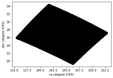
The arguments to plt.plot are x,
y, and a string that specifies the style. In this case, the
letters ko indicate that we want a black, round marker
(k is for black because b is for blue). The
functions xlabel and ylabel put labels on the
axes.
Looking at this plot, we can see that the region we selected, which is a rectangle in GD-1 coordinates, is a non-rectangular region in ICRS coordinates.
However, this scatter plot has a problem. It is “overplotted”, which means that there are so many overlapping points, we cannot distinguish between high and low density areas.
To fix this, we can provide optional arguments to control the size and transparency of the points.
Exercise (5 minutes)
In the call to plt.plot, use the keyword argument
markersize to make the markers smaller.
Then add the keyword argument alpha to make the markers
partly transparent.
Adjust these arguments until you think the figure shows the data most clearly.
Note: Once you have made these changes, you might notice that the figure shows stripes with lower density of stars. These stripes are caused by the way Gaia scans the sky, which you can read about here. The dataset we are using, Gaia Data Release 2, covers 22 months of observations; during this time, some parts of the sky were scanned more than others.
Transform back
Remember that we selected data from a rectangle of coordinates in the GD-1 frame, then transformed them to ICRS when we constructed the query. The coordinates in the query results are in ICRS.
To plot them, we will transform them back to the GD-1 frame; that way, the axes of the figure are aligned with the orbit of GD-1, which is useful for two reasons:
By transforming the coordinates, we can identify stars that are likely to be in GD-1 by selecting stars near the centerline of the stream, where \(\phi_2\) is close to 0.
By transforming the proper motions, we can identify stars with non-zero proper motion along the \(\phi_1\) axis, which are likely to be part of GD-1.
To do the transformation, we will put the results into a
SkyCoord object. In a previous episode, we created a
SkyCoord object like this:
Notice that we did not specify the reference frame. That is because
when using ra and dec in
SkyCoord, the ICRS frame is assumed by
default.
The SkyCoord object can keep track not just of location,
but also proper motions. This means that we can initialize a
SkyCoord object with location and proper motions, then use
all of these quantities together to transform into the GD-1 frame.
Now we are going to do something similar, but now we will take
advantage of the SkyCoord object’s capacity to include and
track space motion information in addition to ra and
dec. We will now also include:
pmraandpmdec, which are proper motion in theICRSframe, anddistanceandradial_velocity, which are important for the reflex correction and will be discussed in that section.
PYTHON
distance = 8 * u.kpc
radial_velocity= 0 * u.km/u.s

skycoord = SkyCoord(ra=polygon_results['ra'],
                    dec=polygon_results['dec'],
                    pm_ra_cosdec=polygon_results['pmra'],
                    pm_dec=polygon_results['pmdec'],
                    distance=distance,
                    radial_velocity=radial_velocity)
For the first four arguments, we use columns from
polygon_results.
For distance and radial_velocity we use
constants, which we explain in the section on reflex correction.
The result is an Astropy SkyCoord object, which we can
transform to the GD-1 frame.
The result is another SkyCoord object, now in the GD-1
frame.
Reflex Correction
The next step is to correct the proper motion measurements for the effect of the motion of our solar system around the Galactic center.
When we created skycoord, we provided constant values
for distance and radial_velocity rather than
measurements from Gaia.
That might seem like a strange thing to do, but here is the motivation:
Because the stars in GD-1 are so far away, parallaxes measured by Gaia are negligible, making the distance estimates unreliable.
So we replace them with our current best estimate of the mean distance to GD-1, about 8 kpc. See Koposov, Rix, and Hogg, 2010.For the other stars in the table, this distance estimate will be inaccurate, so reflex correction will not be correct. But that should have only a small effect on our ability to identify stars with the proper motion we expect for GD-1.
The measurement of radial velocity has no effect on the correction for proper motion, but we have to provide a value to avoid errors in the reflex correction calculation. So we provide
0as an arbitrary place-keeper.
With this preparation, we can use reflex_correct from
Gala (documentation
here) to correct for the motion of the solar system which we have
included as a stand alone file in the student_download.
The result is a SkyCoord object that contains
phi1andphi2, which represent the transformed coordinates in the GD-1 frame.pm_phi1_cosphi2andpm_phi2, which represent the transformed proper motions that have been corrected for the motion of the solar system around the Galactic center.
We can select the coordinates and plot them like this:
PYTHON
x = skycoord_gd1.phi1
y = skycoord_gd1.phi2
plt.plot(x, y, 'ko', markersize=0.1, alpha=0.1)

plt.xlabel('phi1 (degree GD1)')
plt.ylabel('phi2 (degree GD1)')
OUTPUT
<Figure size 432x288 with 1 Axes>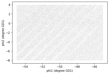
We started with a rectangle in the GD-1 frame. When transformed to the ICRS frame, it is a non-rectangular region. Now, transformed back to the GD-1 frame, it is a rectangle again.
pandas DataFrame
At this point we have two objects containing different sets of the
data relating to identifying stars in GD-1. polygon_results
is the Astropy Table we downloaded from Gaia.
OUTPUT
astropy.table.table.TableAnd skycoord_gd1 is a SkyCoord object that
contains the transformed coordinates and proper motions.
OUTPUT
astropy.coordinates.sky_coordinate.SkyCoordOn one hand, this division of labor makes sense because each object provides different capabilities. But working with multiple object types can be awkward. It will be more convenient to choose one object and get all of the data into it.
Now we can extract the columns we want from skycoord_gd1
and add them to a Pandas DataFrame. phi1 and
phi2 contain the transformed coordinates.
pandas DataFrames versus Astropy
Tables
Two common choices are the pandas DataFrame and Astropy
Table. pandas DataFrames and Astropy
Tables share many of the same characteristics and most of
the manipulations that we do can be done with either. As you become more
familiar with each, you will develop a sense of which one you prefer for
different tasks. For instance you may choose to use Astropy
Tables to read in data, especially astronomy specific data
formats, but pandas DataFrames to inspect the data.
Fortunately, Astropy makes it easy to convert between the two data
types. We will choose to use pandas DataFrame, for two
reasons:
It provides capabilities that are (almost) a superset of the other data structures, so it is the all-in-one solution.
pandas is a general-purpose tool that is useful in many domains, especially data science. If you are going to develop expertise in one tool, pandas is a good choice.
However, compared to an Astropy Table, pandas has one
big drawback: it does not keep the metadata associated with the table,
including the units for the columns. Nevertheless, we think it’s a
useful data type to be familiar with.
It is straightforward to convert an Astropy Table to a
pandas DataFrame.
DataFrame provides shape, which shows the
number of rows and columns.
OUTPUT
(140339, 6)It also provides head, which displays the first few
rows. head is useful for spot-checking large results as you
go along.
OUTPUT
            source_id          ra        dec       pmra       pmdec   parallax
0  637987125186749568  142.483019  21.757716  -2.516838    2.941813  -0.257345
1  638285195917112960  142.254529  22.476168   2.662702  -12.165984   0.422728
2  638073505568978688  142.645286  22.166932  18.306747   -7.950660   0.103640
3  638086386175786752  142.577394  22.227920   0.987786   -2.584105  -0.857327
4  638049655615392384  142.589136  22.110783   0.244439   -4.941079   0.099625
Now we can add the GD-1 coordinates and proper motions as columns in
the DataFrame. We use the .value attribute to
extract the numerical values without units, since Pandas
DataFrames do not preserve astropy units.
PYTHON
results_df['phi1'] = skycoord_gd1.phi1.value
results_df['phi2'] = skycoord_gd1.phi2.value
results_df['pm_phi1'] = skycoord_gd1.pm_phi1_cosphi2.value
results_df['pm_phi2'] = skycoord_gd1.pm_phi2.value
results_df.shape
OUTPUT
(140339, 10)And we can check the result with head:
OUTPUT
            source_id          ra        dec       pmra       pmdec   parallax        phi1       phi2    pm_phi1     pm_phi2
0  637987125186749568  142.483019  21.757716  -2.516838    2.941813  -0.257345  -54.975623  -3.659349   6.429945    6.518157
1  638285195917112960  142.254529  22.476168   2.662702  -12.165984   0.422728  -54.498247  -3.081524  -3.168637   -6.206795
2  638073505568978688  142.645286  22.166932  18.306747   -7.950660   0.103640  -54.551634  -3.554229   9.129447  -16.819570
3  638086386175786752  142.577394  22.227920   0.987786   -2.584105  -0.857327  -54.536457  -3.467966   3.837120    0.526461
4  638049655615392384  142.589136  22.110783   0.244439   -4.941079   0.099625  -54.627448  -3.542738   1.466103   -0.185292
Why .value?
The attributes of a SkyCoord object, like
phi1 and phi2, are Quantity
objects that carry units (for example, degrees). Pandas
DataFrames do not support Quantity columns, so
we use the .value attribute to extract the numerical values
without units.
Detail If you notice that SkyCoord has an attribute
called proper_motion, you might wonder why we are not using
it.
We could have: proper_motion contains the same data as
pm_phi1_cosphi2 and pm_phi2, but in a
different format.
Attributes vs functions
shape is an attribute, so we display its value without
calling it as a function.
head is a function, so we need the parentheses.
Before we go any further, we will take all of the steps that we have
done and consolidate them into a single function that we can use to take
the coordinates and proper motion that we get as an Astropy
Table from our Gaia query, add columns representing the
reflex corrected GD-1 coordinates and proper motions, and transform it
into a pandas DataFrame. This is a general function that we
will use multiple times as we build different queries so we want to
write it once and then call the function rather than having to copy and
paste the code over and over again.
PYTHON
def make_dataframe(table):
    """Transform and astropy table with coords in ICRS, convert to pandas dataframe with GD-1 coordinates.

    table: Astropy Table

    returns: pandas DataFrame
    """
    #Create a SkyCoord object with the coordinates and proper motions
    # in the input table
    skycoord = SkyCoord(
               ra=table['ra'],
               dec=table['dec'],
               pm_ra_cosdec=table['pmra'],
               pm_dec=table['pmdec'],
               distance=8*u.kpc,
               radial_velocity=0*u.km/u.s)

    # Define the GD-1 reference frame
    gd1_frame = GD1Koposov10()

    # Transform input coordinates to the GD-1 reference frame
    transformed = skycoord.transform_to(gd1_frame)

    # Correct GD-1 coordinates for solar system motion around galactic center
    skycoord_gd1 = reflex_correct(transformed)

    # Create DataFrame
    df = table.to_pandas()

    # Add GD-1 reference frame columns for coordinates and proper motions
    df['phi1'] = skycoord_gd1.phi1.value
    df['phi2'] = skycoord_gd1.phi2.value
    df['pm_phi1'] = skycoord_gd1.pm_phi1_cosphi2.value
    df['pm_phi2'] = skycoord_gd1.pm_phi2.value

    return df
Here is how we use the function:
Saving the DataFrame
At this point we have run a successful query and combined the results
into a single DataFrame. This is a good time to save the
data.
To save a pandas DataFrame, one option is to convert it
to an Astropy Table, like this:
PYTHON
from astropy.table import Table

results_table = Table.from_pandas(results_df)
type(results_table)
OUTPUT
astropy.table.table.TableThen we could write the Table to a FITS file, as we did
in the previous lesson.
But, like Astropy, pandas provides functions to write DataFrames in
other formats; to see what they are find
the functions here that begin with to_.
One of the best options is HDF5, which is Version 5 of Hierarchical Data Format.
HDF5 is a binary format, so files are small and fast to read and write (like FITS, but unlike XML).
An HDF5 file is similar to an SQL database in the sense that it can contain more than one table, although in HDF5 vocabulary, a table is called a Dataset. (Multi-extension FITS files can also contain more than one table.)
And HDF5 stores the metadata associated with the table, including column names, row labels, and data types (like FITS).
Finally, HDF5 is a cross-language standard, so if you write an HDF5 file with pandas, you can read it back with many other software tools (more than FITS).
We can write a pandas DataFrame to an HDF5 file like
this:
Because an HDF5 file can contain more than one Dataset, we have to provide a name, or “key”, that identifies the Dataset in the file.
We could use any string as the key, but it is generally a good
practice to use a descriptive name (just like your
DataFrame variable name) so we will give the Dataset in the
file the same name (key) as the DataFrame.
By default, writing a DataFrame appends a new dataset to
an existing HDF5 file. We will use the argument mode='w' to
overwrite the file if it already exists rather than append another
dataset to it.
Summary
In this episode, we re-loaded the Gaia data we saved from a previous query.
We transformed the coordinates and proper motion from ICRS to a frame
aligned with the orbit of GD-1, stored the results in a pandas
DataFrame, and visualized them.
We combined all of these steps into a single function that we can reuse in the future to go straight from the output of a query with object coordinates in the ICRS reference frame directly to a pandas DataFrame that includes object coordinates in the GD-1 reference frame.
We saved our results to an HDF5 file which we can use to restart the analysis from this stage or verify our results at some future time.
- When you make a scatter plot, adjust the size of the markers and their transparency so the figure is not overplotted; otherwise it can misrepresent the data badly.
- For simple scatter plots in Matplotlib,
plotis faster thanscatter. - An Astropy
Tableand a pandasDataFrameare similar in many ways and they provide many of the same functions. They have pros and cons, but for many projects, either one would be a reasonable choice. - To store data from a pandas
DataFrame, a good option is an HDF5 file, which can contain multiple Datasets (we’ll dig in more in the Join lesson).