Coordinate Transformations
Last updated on 2025-12-15 | Edit this page
Overview
Questions
- How do we transform celestial coordinates from one frame to another and save a subset of the results in files?
Objectives
- Use Python string formatting to compose more complex ADQL queries.
- Work with coordinates and other quantities that have units.
- Download the results of a query and store them in a file.
In the previous episode, we wrote ADQL queries and used them to select and download data from the Gaia server. In this episode, we will write a query to select stars from a particular region of the sky.
Outline
We’ll start with an example that does a “cone search”; that is, it selects stars that appear in a circular region of the sky.
Then, to select stars in the vicinity of GD-1, we will:
Use
Quantityobjects to represent measurements with units.Use Astropy to convert coordinates from one frame to another.
Use the ADQL keywords
POLYGON,CONTAINS, andPOINTto select stars that fall within a polygonal region.Submit a query and download the results.
Store the results in a FITS file.
Working with Units
The measurements we will work with are physical quantities, which means that they have two parts, a value and a unit. For example, the coordinate 30° has value 30 and its units are degrees.
Until recently, most scientific computation was done with values only; units were left out of the program altogether, sometimes with catastrophic results.
Astropy provides tools for including units explicitly in computations, which makes it possible to detect errors before they cause disasters.
To use Astropy units, we import them like this:
u is an object that contains most common units and all
SI units.
You can use dir to list them, but you should also read the
documentation.
OUTPUT
['A',
 'AA',
 'AB',
 'ABflux',
 'ABmag',
 'AU',
 'Angstrom',
 'B',
 'Ba',
 'Barye',
 'Bi',
[Output truncated]
To create a quantity, we multiply a value by a unit:
OUTPUT
astropy.units.quantity.QuantityThe result is a Quantity object. Jupyter knows how to
display Quantities like this:
OUTPUT
<Quantity 10. deg>10°
Quantities provides a method called to that
converts to other units. For example, we can compute the number of
arcminutes in angle:
OUTPUT
<Quantity 600. arcmin>600′
If you add quantities, Astropy converts them to compatible units, if possible:
OUTPUT
<Quantity 10.5 deg>10.5°
If the units are not compatible, you get an error. For example:
ERROR
angle + 5 * u.kgcauses a UnitConversionError.
Exercise (5 minutes)
Create a quantity that represents 5 arcminutes
and assign it to a variable called radius.
Then convert it to degrees.
Selecting a Region
One of the most common ways to restrict a query is to select stars in a particular region of the sky. For example, here is a query from the Gaia archive documentation that selects objects in a circular region centered at (88.8, 7.4) with a search radius of 5 arcmin (0.08333 deg).
PYTHON
cone_query = """SELECT
TOP 10
source_id
FROM gaiadr2.gaia_source
WHERE 1=CONTAINS(
  POINT(ra, dec),
  CIRCLE(88.8, 7.4, 0.08333333))
"""
This query uses three keywords that are specific to ADQL (not SQL):
POINT: a location in ICRS coordinates, specified in degrees of right ascension and declination.CIRCLE: a circle where the first two values are the coordinates of the center and the third is the radius in degrees.CONTAINS: a function that returns1if aPOINTis contained in a shape and0otherwise. Here is the documentation ofCONTAINS.
A query like this is called a cone search because it selects stars in a cone. Here is how we run it:
OUTPUT
Created TAP+ (v1.2.1) - Connection:
	Host: gea.esac.esa.int
	Use HTTPS: True
	Port: 443
	SSL Port: 443
Created TAP+ (v1.2.1) - Connection:
	Host: geadata.esac.esa.int
	Use HTTPS: True
	Port: 443
	SSL Port: 443

<astroquery.utils.tap.model.job.Job at 0x7f277785fa30>OUTPUT
<Table length=10>
     source_id
       int64
-------------------
3322773965056065536
3322773758899157120
3322774068134271104
3322773930696320512
3322774377374425728
3322773724537891456
3322773724537891328
[Output truncated]Exercise (5 minutes)
When you are debugging queries like this, you can use
TOP to limit the size of the results, but then you still
don’t know how big the results will be.
An alternative is to use COUNT, which asks for the
number of rows that would be selected, but it does not return them.
In the previous query, replace TOP 10 source_id with
COUNT(source_id) and run the query again. How many stars
has Gaia identified in the cone we searched?
PYTHON
count_cone_query = """SELECT
COUNT(source_id)
FROM gaiadr2.gaia_source
WHERE 1=CONTAINS(
  POINT(ra, dec),
  CIRCLE(88.8, 7.4, 0.08333333))
"""

count_cone_job = Gaia.launch_job(count_cone_query)
count_cone_results = count_cone_job.get_results()
count_cone_results
OUTPUT
<Table length=1>
count
int64
-----
594
Getting GD-1 Data
From the Price-Whelan and Bonaca paper, we will try to reproduce Figure 1, which includes this representation of stars likely to belong to GD-1:
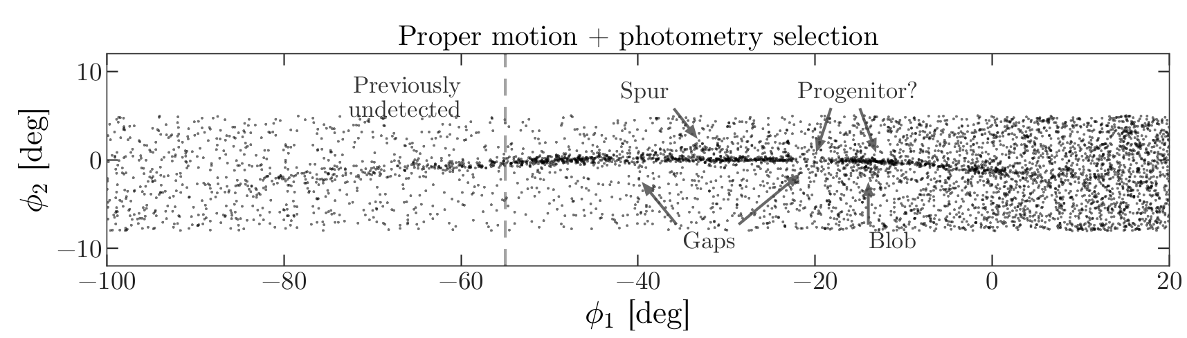
The axes of this figure are defined so the x-axis is aligned with the stars in GD-1, and the y-axis is perpendicular.
Along the x-axis (\(\phi_1\)) the figure extends from -100 to 20 degrees.
Along the y-axis (\(\phi_2\)) the figure extends from about -8 to 4 degrees.
Ideally, we would select all stars from this rectangle, but there are more than 10 million of them. This would be difficult to work with, and as anonymous Gaia users, we are limited to 3 million rows in a single query. While we are developing and testing code, it will be faster to work with a smaller dataset.
So we will start by selecting stars in a smaller rectangle near the center of GD-1, from -55 to -45 degrees \(\phi_1\) and -8 to 4 degrees \(\phi_2\). First we will learn how to represent these coordinates with Astropy.
Transforming coordinates
Astronomy makes use of many different coordinate systems. Transforming between coordinate systems is a common task in observational astronomy, and thankfully, Astropy has abstracted the required spherical trigonometry for us. Below we show the steps to go from Equatorial coordinates (sky coordinates) to Galactic coordinates and finally to a reference frame defined to more easily study GD-1.
Astropy provides a SkyCoord object that represents sky
coordinates relative to a specified reference frame.
The following example creates a SkyCoord object that
represents the approximate coordinates of Betelgeuse
(alf Ori) in the ICRS frame.
ICRS is the “International Celestial Reference System”, adopted in 1997 by the International Astronomical Union.
PYTHON
from astropy.coordinates import SkyCoord

ra = 88.8 * u.degree
dec = 7.4 * u.degree
coord_icrs = SkyCoord(ra=ra, dec=dec, frame='icrs')

coord_icrs
OUTPUT
<SkyCoord (ICRS): (ra, dec) in deg
    (88.8, 7.4)>
SkyCoord objects require units in order to understand
the context. There are a number of ways to define SkyCoord
objects, in our example, we explicitly specified the coordinates and
units and provided a reference frame.
SkyCoord provides the transform_to function
to transform from one reference frame to another reference frame. For
example, we can transform coords_icrs to Galactic
coordinates like this:
OUTPUT
<SkyCoord (Galactic): (l, b) in deg
(199.79693102, -8.95591653)>Coordinate Variables
Notice that in the Galactic frame, the coordinates are the variables
we usually use for Galactic longitude and latitude called l
and b, respectively, not ra and
dec. Most reference frames have different ways to specify
coordinates and the SkyCoord object will use these
names.
To transform to and from GD-1 coordinates, we will use a frame defined by Gala, which is an Astropy-affiliated library that provides tools for galactic dynamics.
Gala provides GD1Koposov10,
which is “a Heliocentric spherical coordinate system defined by the
orbit of the GD-1 stream”. In this coordinate system, one axis is
defined along the direction of the stream (the x-axis in Figure 1) and
one axis is defined perpendicular to the direction of the stream (the
y-axis in Figure 1). These are called the \(\phi_1\) and \(\phi_2\) coordinates, respectively.
OUTPUT
<GD1Koposov10 Frame>GD1Koposov10 import
The GD1Koposov10 reference frame is part of the
gala package. For convience we provide the stand alone file
as part of the student_download zip file you downloaded. If
your notebook is not in your student_download directory,
you will need to add the following before the import statement
Where <path to student_download> is the path to
your student_download directory ending with
student_download.
We can use it to find the coordinates of Betelgeuse in the GD-1 frame, like this:
OUTPUT
<SkyCoord (GD1Koposov10): (phi1, phi2) in deg
(-94.97222038, 34.5813813)>Exercise (10 minutes)
Find the location of GD-1 in ICRS coordinates.
Create a
SkyCoordobject at 0°, 0° in the GD-1 frame.Transform it to the ICRS frame.
Hint: Because ICRS is a standard frame, it is built into Astropy. You
can specify it by name, icrs (as we did with
galactic).
Notice that the origin of the GD-1 frame maps to ra=200,
exactly, in ICRS. That is by design.
Selecting a rectangle
Now that we know how to define coordinate transformations, we are going to use them to get a list of stars that are in GD-1. As we mentioned before, this is a lot of stars, so we are going to start by defining a rectangle that encompasses a small part of GD-1. This is easiest to define in GD-1 coordinates.
The following variables define the boundaries of the rectangle in \(\phi_1\) and \(\phi_2\).
PYTHON
phi1_min = -55 * u.degree
phi1_max = -45 * u.degree
phi2_min = -8 * u.degree
phi2_max = 4 * u.degree
Throughout this lesson we are going to be defining a rectangle often. Rather than copy and paste multiple lines of code, we will write a function to build the rectangle for us. By having the code contained in a single location, we can easily fix bugs or update our implementation as needed. By choosing an explicit function name our code is also self documenting, meaning it’s easy for us to understand that we are building a rectangle when we call this function.
To create a rectangle, we will use the following function, which takes the lower and upper bounds as parameters and returns a list of x and y coordinates of the corners of a rectangle starting with the lower left corner and working clockwise.
PYTHON
def make_rectangle(x1, x2, y1, y2):
    """Return the corners of a rectangle."""
    xs = [x1, x1, x2, x2, x1]
    ys = [y1, y2, y2, y1, y1]
    return xs, ys
The return value is a tuple containing a list of coordinates in \(\phi_1\) followed by a list of coordinates in \(\phi_2\).
phi1_rect and phi2_rect contain the
coordinates of the corners of a rectangle in the GD-1 frame.
While it is easier to visualize the regions we want to define in the GD-1 frame, the coordinates in the Gaia catalog are in the ICRS frame. In order to use the rectangle we defined, we need to convert the coordinates from the GD-1 frame to the ICRS frame. We will do this using the SkyCoord object. Fortunately SkyCoord objects can take lists of coordinates, in addition to single values.
OUTPUT
<SkyCoord (GD1Koposov10): (phi1, phi2) in deg
    [(-55., -8.), (-55.,  4.), (-45.,  4.), (-45., -8.), (-55., -8.)]>
Now we can use transform_to to convert to ICRS
coordinates.
OUTPUT
<SkyCoord (ICRS): (ra, dec) in deg
    [(146.27533314, 19.26190982), (135.42163944, 25.87738723),
     (141.60264825, 34.3048303 ), (152.81671045, 27.13611254),
     (146.27533314, 19.26190982)]>
Notice that a rectangle in one coordinate system is not necessarily a rectangle in another. In this example, the result is a (non-rectangular) polygon. This is why we defined our rectangle in the GD-1 frame.
Defining a polygon
In order to use this polygon as part of an ADQL query, we have to convert it to a string with a comma-separated list of coordinates, as in this example:
SkyCoord provides to_string, which produces
a list of strings.
OUTPUT
['146.275 19.2619',
 '135.422 25.8774',
 '141.603 34.3048',
 '152.817 27.1361',
 '146.275 19.2619']
We can use the Python string function join to join
corners_list_str into a single string (with spaces between
the pairs):
OUTPUT
'146.275 19.2619 135.422 25.8774 141.603 34.3048 152.817 27.1361 146.275 19.2619'This is almost what we need, but we have to replace the spaces with commas.
OUTPUT
'146.275, 19.2619, 135.422, 25.8774, 141.603, 34.3048, 152.817, 27.1361, 146.275, 19.2619'This is something we will need to do multiple times. We will write a function to do it for us so we don’t have to copy and paste every time. The following function combines these steps.
PYTHON
def skycoord_to_string(skycoord):
    """Convert a one-dimensional list of SkyCoord to string for Gaia's query format."""
    corners_list_str = skycoord.to_string()
    corners_single_str = ' '.join(corners_list_str)
    return corners_single_str.replace(' ', ', ')
Here is how we use this function:
OUTPUT
'146.275, 19.2619, 135.422, 25.8774, 141.603, 34.3048, 152.817, 27.1361, 146.275, 19.2619'Assembling the query
Now we are ready to assemble our query to get all of the stars in the Gaia catalog that are in the small rectangle we defined and are likely to be part of GD-1 with the criteria we previously defined.
We need columns again (as we saw in the previous
episode).
And here is the query base we used in the previous lesson:
PYTHON
query3_base = """SELECT
TOP 10
{columns}
FROM gaiadr2.gaia_source
WHERE parallax < 1
  AND bp_rp BETWEEN -0.75 AND 2
"""
Now we will add a WHERE clause to select stars in the
polygon we defined and start using more descriptive variables for our
queries.
PYTHON
polygon_top10query_base = """SELECT
TOP 10
{columns}
FROM gaiadr2.gaia_source
WHERE parallax < 1
  AND bp_rp BETWEEN -0.75 AND 2
  AND 1 = CONTAINS(POINT(ra, dec),
                   POLYGON({sky_point_list}))
"""
The query base contains format specifiers for columns
and sky_point_list.
We will use format to fill in these values.
PYTHON
polygon_top10query = polygon_top10query_base.format(columns=columns,
                          sky_point_list=sky_point_list)
print(polygon_top10query)
OUTPUT
SELECT
TOP 10
source_id, ra, dec, pmra, pmdec, parallax
FROM gaiadr2.gaia_source
WHERE parallax < 1
  AND bp_rp BETWEEN -0.75 AND 2
  AND 1 = CONTAINS(POINT(ra, dec),
                   POLYGON(146.275, 19.2619, 135.422, 25.8774, 141.603, 34.3048, 152.817, 27.1361, 146.275, 19.2619))
As always, we should take a minute to proof-read the query before we launch it.
PYTHON
polygon_top10query_job = Gaia.launch_job_async(polygon_top10query)
print(polygon_top10query_job)
OUTPUT
INFO: Query finished. [astroquery.utils.tap.core]
<Table length=10>
   name    dtype    unit                              description
--------- ------- -------- ------------------------------------------------------------------
source_id   int64          Unique source identifier (unique within a particular Data Release)
       ra float64      deg                                                    Right ascension
      dec float64      deg                                                        Declination
     pmra float64 mas / yr                         Proper motion in right ascension direction
    pmdec float64 mas / yr                             Proper motion in declination direction
 parallax float64      mas                                                           Parallax
Jobid: 1615815873808O
Phase: COMPLETED
[Output truncated]
Here are the results.
OUTPUT
<Table length=10>
    source_id              ra         ...       parallax
                          deg         ...         mas
------------------ ------------------ ... --------------------
637987125186749568 142.48301935991023 ...  -0.2573448962333354
638285195917112960 142.25452941346344 ...   0.4227283465319491
638073505568978688 142.64528557468074 ...  0.10363972229362585
638086386175786752 142.57739430926034 ...  -0.8573270355079308
638049655615392384 142.58913564478618 ...    0.099624729200593
638267565075964032 141.81762228999614 ... -0.07271215219283075
[Output truncated]
Finally, we can remove TOP 10 and run the query
again.
The result is bigger than our previous queries, so it will take a little longer.
PYTHON
polygon_query_base = """SELECT
{columns}
FROM gaiadr2.gaia_source
WHERE parallax < 1
  AND bp_rp BETWEEN -0.75 AND 2
  AND 1 = CONTAINS(POINT(ra, dec),
                   POLYGON({sky_point_list}))
"""
PYTHON
polygon_query = polygon_query_base.format(columns=columns,
                          sky_point_list=sky_point_list)
print(polygon_query)
OUTPUT
SELECT
source_id, ra, dec, pmra, pmdec, parallax
FROM gaiadr2.gaia_source
WHERE parallax < 1
  AND bp_rp BETWEEN -0.75 AND 2
  AND 1 = CONTAINS(POINT(ra, dec),
POLYGON(146.275, 19.2619, 135.422, 25.8774, 141.603, 34.3048, 152.817, 27.1361, 146.275, 19.2619))OUTPUT
INFO: Query finished. [astroquery.utils.tap.core]
<Table length=140339>
   name    dtype    unit                              description
--------- ------- -------- ------------------------------------------------------------------
source_id   int64          Unique source identifier (unique within a particular Data Release)
       ra float64      deg                                                    Right ascension
      dec float64      deg                                                        Declination
     pmra float64 mas / yr                         Proper motion in right ascension direction
    pmdec float64 mas / yr                             Proper motion in declination direction
 parallax float64      mas                                                           Parallax
Jobid: 1615815886707O
Phase: COMPLETED
[Output truncated]OUTPUT
140339There are more than 100,000 stars in this polygon, but that’s a manageable size to work with.
Saving results
This is the set of stars we will work with in the next step. Since we have a substantial dataset now, this is a good time to save it.
Storing the data in a file means we can shut down our notebook and pick up where we left off without running the previous query again.
Astropy Table objects provide write, which
writes the table to disk.
Because the filename ends with fits, the table is
written in the FITS
format, which preserves the metadata associated with the table.
If the file already exists, the overwrite argument
causes it to be overwritten.
We can use getsize to confirm that the file exists and
check the size:
OUTPUT
6.4324951171875Summary
In this notebook, we composed more complex queries to select stars within a polygonal region of the sky. Then we downloaded the results and saved them in a FITS file.
In the next notebook, we’ll reload the data from this file and replicate the next step in the analysis, using proper motion to identify stars likely to be in GD-1.
- For measurements with units, use
Quantityobjects that represent units explicitly and check for errors. - Use the
formatfunction to compose queries; it is often faster and less error-prone. - Develop queries incrementally: start with something simple, test it, and add a little bit at a time.
- Once you have a query working, save the data in a local file. If you shut down the notebook and come back to it later, you can reload the file; you don’t have to run the query again.