Join
Last updated on 2026-06-19 | Edit this page
Overview
Questions
- How do we use
JOINto combine information from multiple tables? - How can we make a selection within a joined table?
- How should we save the result?
Objectives
- Write ADQL queries involving
JOINoperations. - Save data in CSV format.
The next step in our analysis is to select candidate stars based on photometry data. The following figure from the Price-Whelan and Bonaca paper is a color-magnitude diagram for the stars selected based on proper motion:
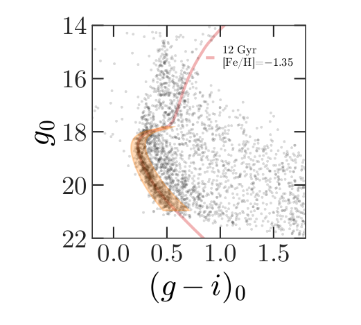
In red is a stellar isochrone, showing where we expect the stars in GD-1 to fall based on the metallicity and age of their original globular cluster.
By selecting stars in the shaded area, we can further distinguish the main sequence of GD-1 from younger background stars.
Outline
We will reload the candidate stars we identified in the previous episode.
Then we will run a query on the Gaia server that uploads the table of candidates and uses a
JOINoperation to select photometry data for the candidate stars.We will write the results to a file for use in the next episode.
Starting from this episode
If you are starting a new notebook for this episode, expand this section for information you will need to get started.
In the previous episode, we define a rectangle around stars in GD-1 in spatial coordinates and in proper motion which we transformed into ICRS coordinates and created point lists of the polygon vertices. We will use that data for this episode. Whether you are working from a new notebook or coming back from a checkpoint, reloading the data will save you from having to run the query again.
If you are starting this episode here or starting this episode in a new notebook, you will need run the following lines of code.
This imports previously imported functions:
The following code loads in the data (instructions for downloading
data can be found in the setup instructions).
You may need to add a the path to the filename variable below
(e.g. filename = 'student_download/backup-data/gd1_data.hdf')
Getting photometry data
The Gaia dataset contains some photometry data, including the
variable bp_rp, which contains BP-RP color (the difference
in mean flux between the BP and RP bands). We use this variable to
select stars with bp_rp between -0.75 and 2, which excludes
many class M dwarf stars.
But we can do better than that. Assuming GD-1 is a globular cluster,
all of the stars formed at the same time from the same material, so the
stars’ photometric properties should be consistent with a single
isochrone in a color magnitude diagram. We can use photometric color and
apparent magnitude to select stars with the age and metal richness we
expect in GD-1. However, the broad Gaia photometric bands (G, BP, RP)
are not optimized for this task, instead we will use the more narrow
photometric bands available from the Pan-STARRS survey to obtain the
g-i color and apparent g-band magnitude.
Conveniently, the Gaia server provides data from Pan-STARRS as a table in the same database we have been using, so we can access it by making ADQL queries.
A caveat about matching stars between catalogs
In general, choosing a star from the Gaia catalog and finding the corresponding star in the Pan-STARRS catalog is not easy. This kind of cross matching is not always possible, because a star might appear in one catalog and not the other. And even when both stars are present, there might not be a clear one-to-one relationship between stars in the two catalogs. Additional catalog matching tools are available from the Astropy coordinates package.
Fortunately, people have worked on this problem, and the Gaia database includes cross-matching tables that suggest a best neighbor in the Pan-STARRS catalog for many stars in the Gaia catalog.
This document describes the cross matching process. Briefly, it uses a cone search to find possible matches in approximately the right position, then uses attributes like color and magnitude to choose pairs of observations most likely to be the same star.
The best neighbor table
So the hard part of cross-matching has been done for us. Using the results is a little tricky, but it gives us a chance to learn about one of the most important tools for working with databases: “joining” tables.
A “join” is an operation where you match up records from one table with records from another table using as a “key” a piece of information that is common to both tables, usually some kind of ID code.
In this example:
Stars in the Gaia dataset are identified by
source_id.Stars in the Pan-STARRS dataset are identified by
obj_id.
For each candidate star we have selected so far, we have the
source_id; the goal is to find the obj_id for
the same star in the Pan-STARRS catalog.
To do that we will:
Use the
JOINoperator to look up each Pan-STARRSobj_id, for the stars we are interested in, in thepanstarrs1_best_neighbourtable using thesource_idsthat we have already identified.Use the
JOINoperator again to look up the Pan-STARRS photometry for these stars in thepanstarrs1_original_validtable using theobj_idswe just identified.
Before we get to the JOIN operation, we will explore
these tables.
British vs American Spelling of Neighbour
The Gaia database was created and is maintained by the European Space Astronomy Center. For this reason, the table spellings use the British spelling of neighbour (with a “u”). Do not forget to include it in your table names in the queries below.
Here is the metadata for panstarrs1_best_neighbour.
OUTPUT
TAP Table name: gaiadr2.gaiadr2.panstarrs1_best_neighbour
Description: Pan-STARRS1 BestNeighbour table lists each matched Gaia object with its
best neighbour in the external catalogue.
There are 1 327 157 objects in the filtered version of Pan-STARRS1 used
to compute this cross-match that have too early epochMean.
Size (bytes): 98462015488
Num. columns: 7
And here are the columns.
OUTPUT
source_id
original_ext_source_id
angular_distance
number_of_neighbours
number_of_mates
best_neighbour_multiplicity
gaia_astrometric_params
Here is the documentation for these variables.
The ones we will use are:
source_id, which we will match up withsource_idin the Gaia table.best_neighbour_multiplicity, which indicates how many sources in Pan-STARRS are matched with the same probability to this source in Gaia.number_of_mates, which indicates the number of other sources in Gaia that are matched with the same source in Pan-STARRS.original_ext_source_id, which we will match up withobj_idin the Pan-STARRS table.
Ideally, best_neighbour_multiplicity should be 1 and
number_of_mates should be 0; in that case, there is a
one-to-one match between the source in Gaia and the corresponding source
in Pan-STARRS.
Number of neighbors
The table also contains number_of_neighbours which is
the number of stars in Pan-STARRS that match in terms of position,
before using other criteria to choose the most likely match. But we are
more interested in the final match, using both criteria.
Here is a query that selects these columns and returns the first 5 rows.
PYTHON
ps_best_neighbour_query = """SELECT
TOP 5
source_id, best_neighbour_multiplicity, number_of_mates, original_ext_source_id
FROM gaiadr2.panstarrs1_best_neighbour
"""OUTPUT
INFO: Query finished. [astroquery.utils.tap.core]OUTPUT
<Table length=5>
     source_id      best_neighbour_multiplicity number_of_mates original_ext_source_id
       int64                  int32                  int16              int64
------------------- --------------------------- --------------- ----------------------
6745938972433480704                           1               0      69742925668851205
6030466788955954048                           1               0      69742509325691172
6756488099308169600                           1               0      69742879438541228
6700154994715046016                           1               0      69743055581721207
6757061941303252736                           1               0      69742856540241198
The Pan-STARRS table
Now that we know the Pan-STARRS obj_id, we are ready to
match this to the photometry in the
panstarrs1_original_valid table. Here is the metadata for
the table that contains the Pan-STARRS data.
OUTPUT
TAP Table name: gaiadr2.gaiadr2.panstarrs1_original_valid
Description: The Panoramic Survey Telescope and Rapid Response System (Pan-STARRS) is
a system for wide-field astronomical imaging developed and operated by
the Institute for Astronomy at the University of Hawaii. Pan-STARRS1
(PS1) is the first part of Pan-STARRS to be completed and is the basis
for Data Release 1 (DR1). The PS1 survey used a 1.8 meter telescope and
its 1.4 Gigapixel camera to image the sky in five broadband filters (g,
r, i, z, y).

The current table contains a filtered subsample of the 10 723 304 629
entries listed in the original ObjectThin table.
[Output truncated]
And here are the columns.
OUTPUT
obj_name
obj_id
ra
dec
ra_error
dec_error
epoch_mean
g_mean_psf_mag
g_mean_psf_mag_error
g_flags
r_mean_psf_mag
[Output truncated]
Here is the documentation for these variables .
The ones we will use are:
obj_id, which we will match up withoriginal_ext_source_idin the best neighbor table.g_mean_psf_mag, which contains mean magnitude from thegfilter.i_mean_psf_mag, which contains mean magnitude from theifilter.
Here is a query that selects these variables and returns the first 5 rows.
PYTHON
ps_valid_query = """SELECT
TOP 5
obj_id, g_mean_psf_mag, i_mean_psf_mag
FROM gaiadr2.panstarrs1_original_valid
"""OUTPUT
INFO: Query finished. [astroquery.utils.tap.core]OUTPUT
<Table length=5>
      obj_id      g_mean_psf_mag  i_mean_psf_mag
                                       mag
      int64          float64         float64
----------------- -------------- ----------------
67130655389101425             -- 20.3516006469727
67553305590067819             --  19.779899597168
67551423248967849             -- 19.8889007568359
67132026238911331             -- 20.9062995910645
67553513677687787             -- 21.2831001281738
Joining tables
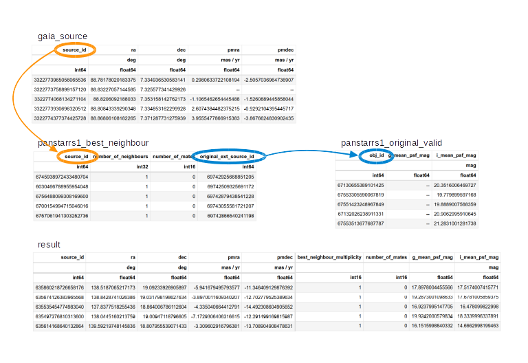
The following figure shows how these tables are related.
The orange circles and arrows represent the first
JOINoperation, which takes eachsource_idin the Gaia table and finds the same value ofsource_idin the best neighbor table.The blue circles and arrows represent the second
JOINoperation, which takes eachoriginal_ext_source_idin the best neighbor table and finds the same value ofobj_idin the PanSTARRS photometry table.
There is no guarantee that the corresponding rows of these tables are
in the same order, so the JOIN operation involves some
searching. However, ADQL/SQL databases are implemented in a way that
makes this kind of search efficient. If you are curious, you can read
more about it.
Now we will get to the details of performing a JOIN
operation.
We are about to build a complex query using software that doesn’t provide us with any helpful information for debugging. For this reason we are going to start with a simplified version of what we want to do until we are sure we are joining the tables correctly, then we will slowly add more layers of complexity, checking at each stage that our query still works. As a starting place, we will go all the way back to the cone search from episode 2.
PYTHON
test_cone_query = """SELECT
TOP 10
source_id
FROM gaiadr2.gaia_source
WHERE 1=CONTAINS(
  POINT(ra, dec),
  CIRCLE(88.8, 7.4, 0.08333333))
"""
And we will run it, to make sure we have a working query to build on.
OUTPUT
INFO: Query finished. [astroquery.utils.tap.core]OUTPUT
<Table length=10>
     source_id
       int64
-------------------
3322773965056065536
3322773758899157120
3322774068134271104
3322773930696320512
3322774377374425728
3322773724537891456
3322773724537891328
[Output truncated]
Now we can start adding features. First, we will replace
source_id with the format specifier columns so
that we can alter what columns we want to return without having to
modify our base query:
PYTHON
cone_base_query = """SELECT
{columns}
FROM gaiadr2.gaia_source
WHERE 1=CONTAINS(
  POINT(ra, dec),
  CIRCLE(88.8, 7.4, 0.08333333))
"""
As a reminder, here are the columns we want from the Gaia table:
PYTHON
columns = 'source_id, ra, dec, pmra, pmdec'

cone_query = cone_base_query.format(columns=columns)
print(cone_query)
OUTPUT
SELECT
source_id, ra, dec, pmra, pmdec
FROM gaiadr2.gaia_source
WHERE 1=CONTAINS(
  POINT(ra, dec),
  CIRCLE(88.8, 7.4, 0.08333333))
We run the query again.
OUTPUT
INFO: Query finished. [astroquery.utils.tap.core]OUTPUT
<Table length=594>
     source_id              ra        ...        pmdec
                           deg        ...       mas / yr
       int64             float64      ...       float64
------------------- ----------------- ... -------------------
3322773965056065536 88.78178020183375 ... -2.5057036964736907
3322773758899157120 88.83227057144585 ...                  --
3322774068134271104  88.8206092188033 ... -1.5260889445858044
3322773930696320512 88.80843339290348 ... -0.9292104395445717
3322774377374425728 88.86806108182265 ... -3.8676624830902435
3322773724537891456 88.81308602813434 ... -33.078133430952086
[Output truncated]
Adding the best neighbor table
Now we are ready for the first join. The join operation requires two clauses:
JOINspecifies the name of the table we want to join with, andONspecifies how we will match up rows between the tables.
In this example, we join with
gaiadr2.panstarrs1_best_neighbour AS best, which means we
can refer to the best neighbor table with the abbreviated name
best, which will save us a lot of typing. Similarly, we
will be referring to the gaiadr2.gaia_source table by the
abbreviated name gaia.
The ON clause indicates that we will match up the
source_id column from the Gaia table with the
source_id column from the best neighbor table.
PYTHON
neighbours_base_query = """SELECT
{columns}
FROM gaiadr2.gaia_source AS gaia
JOIN gaiadr2.panstarrs1_best_neighbour AS best
  ON gaia.source_id = best.source_id
WHERE 1=CONTAINS(
  POINT(gaia.ra, gaia.dec),
  CIRCLE(88.8, 7.4, 0.08333333))
"""SQL detail
In this example, the ON column has the same name in both
tables, so we could replace the ON clause with a simpler USINGclause:
Now that there is more than one table involved, we can’t use simple
column names any more; we have to use qualified column
names. In other words, we have to specify which table each
column is in. The column names do not have to be the same and, in fact,
in the next join they will not be. That is one of the reasons that we
explicitly specify them. Here is the complete query, including the
columns we want from the Gaia and best neighbor tables. Here you can
start to see that using the abbreviated names is making our query easier
to read and requires less typing for us. In addition to the spatial
coordinates and proper motion, we are going to return the
best_neighbour_multiplicity and
number_of_mates columns from the
panstarrs1_best_neighbour table in order to evaluate the
quality of the data that we are using by evaluating the number of
one-to-one matches between the catalogs. Recall that
best_neighbour_multiplicity tells us the number of
PanSTARRs objects that match a Gaia object and
number_of_mates tells us the number of Gaia objects that
match a PanSTARRs object.
PYTHON
column_list_neighbours = ['gaia.source_id',
               'gaia.ra',
               'gaia.dec',
               'gaia.pmra',
               'gaia.pmdec',
               'best.best_neighbour_multiplicity',
               'best.number_of_mates',
              ]
columns = ', '.join(column_list_neighbours)

neighbours_query = neighbours_base_query.format(columns=columns)
print(neighbours_query)
OUTPUT
SELECT
gaia.source_id, gaia.ra, gaia.dec, gaia.pmra, gaia.pmdec, best.best_neighbour_multiplicity, best.number_of_mates
FROM gaiadr2.gaia_source AS gaia
JOIN gaiadr2.panstarrs1_best_neighbour AS best
  ON gaia.source_id = best.source_id
WHERE 1=CONTAINS(
  POINT(gaia.ra, gaia.dec),
CIRCLE(88.8, 7.4, 0.08333333))OUTPUT
INFO: Query finished. [astroquery.utils.tap.core]OUTPUT
<Table length=490>
     source_id              ra        ... number_of_mates
                           deg        ...
       int64             float64      ...      int16
------------------- ----------------- ... ---------------
3322773965056065536 88.78178020183375 ...               0
3322774068134271104  88.8206092188033 ...               0
3322773930696320512 88.80843339290348 ...               0
3322774377374425728 88.86806108182265 ...               0
3322773724537891456 88.81308602813434 ...               0
3322773724537891328 88.81570329208743 ...               0
[Output truncated]
This result has fewer rows than the previous result. That is because there are sources in the Gaia table with no corresponding source in the Pan-STARRS table.
By default, the result of the join only includes rows where the same
source_id appears in both tables. This default is called an
“inner” join because the results include only the intersection of the
two tables. You
can read about the other kinds of join here.
Adding the Pan-STARRS table
Exercise (15 minutes)
Now we are ready to bring in the Pan-STARRS table. Starting with the
previous query, add a second JOIN clause that joins with
gaiadr2.panstarrs1_original_valid, gives it the abbreviated
name ps, and matches original_ext_source_id
from the best neighbor table with obj_id from the
Pan-STARRS table.
Add g_mean_psf_mag and i_mean_psf_mag to
the column list, and run the query. The result should contain 490 rows
and 9 columns.
PYTHON
join_solution_query_base = """SELECT
{columns}
FROM gaiadr2.gaia_source as gaia
JOIN gaiadr2.panstarrs1_best_neighbour as best
  ON gaia.source_id = best.source_id
JOIN gaiadr2.panstarrs1_original_valid as ps
  ON best.original_ext_source_id = ps.obj_id
WHERE 1=CONTAINS(
  POINT(gaia.ra, gaia.dec),
  CIRCLE(88.8, 7.4, 0.08333333))
"""

column_list = ['gaia.source_id',
               'gaia.ra',
               'gaia.dec',
               'gaia.pmra',
               'gaia.pmdec',
               'best.best_neighbour_multiplicity',
               'best.number_of_mates',
               'ps.g_mean_psf_mag',
               'ps.i_mean_psf_mag']

columns = ', '.join(column_list)

join_solution_query = join_solution_query_base.format(columns=columns)
print(join_solution_query)

join_solution_job = Gaia.launch_job_async(join_solution_query)
join_solution_results = join_solution_job.get_results()
join_solution_results
OUTPUT
<Table length=490>
     source_id              ra        ...  g_mean_psf_mag   i_mean_psf_mag
                           deg        ...                        mag
       int64             float64      ...     float64          float64
------------------- ----------------- ... ---------------- ----------------
3322773965056065536 88.78178020183375 ... 19.9431991577148 17.4221992492676
3322774068134271104  88.8206092188033 ... 18.6212005615234 16.6007995605469
3322773930696320512 88.80843339290348 ...               -- 20.2203998565674
3322774377374425728 88.86806108182265 ... 18.0676002502441 16.9762001037598
3322773724537891456 88.81308602813434 ... 20.1907005310059 17.8700008392334
3322773724537891328 88.81570329208743 ... 22.6308002471924 19.6004009246826
[Output truncated]
Selecting by coordinates and proper motion
We are now going to replace the cone search with the GD-1 selection
that we built in previous episodes. We will start by making sure that
our previous query works, then add in the JOIN. Now we will
bring in the WHERE clause from the previous episode, which
selects sources based on parallax, BP-RP color, sky coordinates, and
proper motion.
Here is candidate_coord_pm_query_base from the previous
episode.
PYTHON
candidate_coord_pm_query_base = """SELECT
{columns}
FROM gaiadr2.gaia_source
WHERE parallax < 1
  AND bp_rp BETWEEN -0.75 AND 2
  AND 1 = CONTAINS(POINT(ra, dec),
                   POLYGON({sky_point_list}))
  AND pmra BETWEEN {pmra_min} AND  {pmra_max}
  AND pmdec BETWEEN {pmdec_min} AND {pmdec_max}
"""
Now we can assemble the query using the sky point list and proper motion range we compiled in episode 5.
PYTHON
columns = 'source_id, ra, dec, pmra, pmdec'

candidate_coord_pm_query = candidate_coord_pm_query_base.format(columns=columns,
                            sky_point_list=sky_point_list,
                            pmra_min=pmra_min,
                            pmra_max=pmra_max,
                            pmdec_min=pmdec_min,
                            pmdec_max=pmdec_max)

print(candidate_coord_pm_query)
OUTPUT
SELECT
source_id, ra, dec, pmra, pmdec
FROM gaiadr2.gaia_source
WHERE parallax < 1
  AND bp_rp BETWEEN -0.75 AND 2
  AND 1 = CONTAINS(POINT(ra, dec),
                   POLYGON(135.306, 8.39862, 126.51, 13.4449, 163.017, 54.2424, 172.933, 46.4726, 135.306, 8.39862))
  AND pmra BETWEEN -6.70 AND -3
  AND pmdec BETWEEN -14.31 AND -11.2
We run it to make sure we are starting with a working query.
OUTPUT
INFO: Query finished. [astroquery.utils.tap.core]OUTPUT
<Table length=8409>
    source_id              ra         ...        pmdec
                          deg         ...       mas / yr
      int64             float64       ...       float64
------------------ ------------------ ... -------------------
635559124339440000 137.58671691646745 ... -12.490481778113859
635860218726658176  138.5187065217173 ... -11.346409129876392
635674126383965568  138.8428741026386 ... -12.702779525389634
635535454774983040  137.8377518255436 ... -14.492308604905652
635497276810313600  138.0445160213759 ... -12.291499169815987
635614168640132864 139.59219748145836 ... -13.708904908478631
[Output truncated]Exercise (15 minutes)
Create a new query base called candidate_join_query_base
that combines the WHERE clauses from the previous query
with the JOIN clauses for the best neighbor and Pan-STARRS
tables. Format the query base using the column names in
column_list, and call the result
candidate_join_query.
Hint: Make sure you use qualified column names everywhere!
Run your query and download the results. The table you get should have 4300 rows and 9 columns.
PYTHON
candidate_join_query_base = """
SELECT
{columns}
FROM gaiadr2.gaia_source as gaia
JOIN gaiadr2.panstarrs1_best_neighbour as best
  ON gaia.source_id = best.source_id
JOIN gaiadr2.panstarrs1_original_valid as ps
  ON best.original_ext_source_id = ps.obj_id
WHERE parallax < 1
  AND bp_rp BETWEEN -0.75 AND 2
  AND 1 = CONTAINS(POINT(gaia.ra, gaia.dec),
                   POLYGON({sky_point_list}))
  AND gaia.pmra BETWEEN {pmra_min} AND  {pmra_max}
  AND gaia.pmdec BETWEEN {pmdec_min} AND {pmdec_max}
"""

columns = ', '.join(column_list)

candidate_join_query = candidate_join_query_base.format(columns=columns,
                            sky_point_list= sky_point_list,
                            pmra_min=pmra_min,
                            pmra_max=pmra_max,
                            pmdec_min=pmdec_min,
                            pmdec_max=pmdec_max)
print(candidate_join_query)


candidate_join_job = Gaia.launch_job_async(candidate_join_query)
candidate_table = candidate_join_job.get_results()
candidate_table
Checking the match
To get more information about the matching process, we can inspect
best_neighbour_multiplicity, which indicates for each star
in Gaia how many stars in Pan-STARRS are equally likely matches.
OUTPUT
<MaskedColumn name='best_neighbour_multiplicity' dtype='int16' description='Number of neighbours with same probability as best neighbour' length=4300>
  1
  1
  1
  1
  1
  1
  1
  1
  1
  1
[Output truncated]
Most of the values are 1, which is good; that means that
for each candidate star we have identified exactly one source in
Pan-STARRS that is likely to be the same star.
To check whether there are any values other than 1, we
can convert this column to a pandas Series and use
describe, which we saw in episode 3.
PYTHON
multiplicity = pd.Series(candidate_table['best_neighbour_multiplicity'])
multiplicity.describe()
OUTPUT
count    4300.0
mean        1.0
std         0.0
min         1.0
25%         1.0
50%         1.0
75%         1.0
max         1.0
dtype: float64
In fact, 1 is the only value in the Series,
so every candidate star has a single best match.
Numpy Mask Warning
You may see a warning that ends with the following phrase:
site-packages/numpy/lib/function_base.py:4650:
UserWarning: Warning: 'partition' will ignore the 'mask' of the MaskedColumn.
arr.partition(
This is because astroquery is returning a table with masked columns (which are really fancy masked numpy arrays). When we turn this column into a pandas Series, it maintains its mask. Describe calls numpy functions to perform statistics. Numpy recently implemented this warning to let you know that the mask is not being considered in the calculation its performing.
Similarly, number_of_mates indicates the number of
other stars in Gaia that match with the same star in
Pan-STARRS.
OUTPUT
count    4300.0
mean        0.0
std         0.0
min         0.0
25%         0.0
50%         0.0
75%         0.0
max         0.0
dtype: float64
All values in this column are 0, which means that for
each match we found in Pan-STARRS, there are no other stars in Gaia that
also match.
Saving the DataFrame
We can make a DataFrame from our Astropy
Table and save our results so we can pick up where we left
off without running this query again. Once again, we will make use of
our make_dataframe function.
The HDF5 file should already exist, so we’ll add
candidate_df to it.
We can use getsize to confirm that the file exists and
check the size:
OUTPUT
15.422508239746094Another file format - CSV
pandas can write a variety of other formats, which you can read about here. We won’t cover all of them, but one other important one is CSV, which stands for “comma-separated values”.
CSV is a plain-text format that can be read and written by pretty much any tool that works with data. In that sense, it is the “least common denominator” of data formats.
However, it has an important limitation: some information about the data gets lost in translation, notably the data types. If you read a CSV file from someone else, you might need some additional information to make sure you are getting it right.
Also, CSV files tend to be big, and slow to read and write.
With those caveats, here is how to write one:
We can check the file size like this:
OUTPUT
0.8787498474121094We can read the CSV file back like this:
We will compare the first few rows of candidate_df and
read_back_csv
OUTPUT
            source_id          ra        dec      pmra      pmdec  \
0  635860218726658176  138.518707  19.092339 -5.941679 -11.346409
1  635674126383965568  138.842874  19.031798 -3.897001 -12.702780
2  635535454774983040  137.837752  18.864007 -4.335041 -14.492309

   best_neighbour_multiplicity  number_of_mates  g_mean_psf_mag  \
0                            1                0         17.8978
1                            1                0         19.2873
2                            1                0         16.9238

   i_mean_psf_mag       phi1      phi2   pm_phi1   pm_phi2
[Output truncated]OUTPUT
   Unnamed: 0           source_id          ra        dec      pmra      pmdec  \
0           0  635860218726658176  138.518707  19.092339 -5.941679 -11.346409
1           1  635674126383965568  138.842874  19.031798 -3.897001 -12.702780
2           2  635535454774983040  137.837752  18.864007 -4.335041 -14.492309

   best_neighbour_multiplicity  number_of_mates  g_mean_psf_mag  \
0                            1                0         17.8978
1                            1                0         19.2873
2                            1                0         16.9238

   i_mean_psf_mag       phi1      phi2   pm_phi1   pm_phi2
[Output truncated]
The CSV file contains the names of the columns, but not the data
types. A keen observer may note that the dataframe that we
wrote to the CSV file did not contain data types, so it is unsurprising
that the CSV file also does not. However, even if we had written a CSV
file from an astropy Table, which does contain data type,
data type would not appear in the CSV file, highlighting a limitation of
this format. Additionally, notice that the index in
candidate_df has become an unnamed column in
read_back_csv and a new index has been created. The pandas
functions for writing and reading CSV files provide options to avoid
that problem, but this is an example of the kind of thing that can go
wrong with CSV files.
Summary
In this episode, we used database JOIN operations to
select photometry data for the stars we’ve identified as candidates to
be in GD-1.
In the next episode, we will use this data for a second round of selection, identifying stars that have photometry data consistent with GD-1.
- Use
JOINoperations to combine data from multiple tables in a database, using some kind of identifier to match up records from one table with records from another. This is another example of a practice we saw in the previous notebook, moving the computation to the data. - For most applications, saving data in FITS or HDF5 is better than CSV. FITS and HDF5 are binary formats, so the files are usually smaller, and they store metadata, so you don’t lose anything when you read the file back.
- On the other hand, CSV is a ‘least common denominator’ format; that is, it can be read by practically any application that works with data.