Transform and Select

Overview

Questions

• When should we use the database server for computation?
• When should we download the data from the database server and compute locally?

Objectives

• Transform proper motions from one frame to another.
• Compute the convex hull of a set of points.
• Write an ADQL query that selects based on proper motion.

In the previous episode, we identified stars with the proper motion we expect for GD-1.

Now we will do the same selection in an ADQL query, which will make it possible to work with a larger region of the sky and still download less data.

Outline

1. Using data from the previous episode, we will identify the values of proper motion for stars likely to be in GD-1.

2. Then we will compose an ADQL query that selects stars based on proper motion, so we can download only the data we need.

That will make it possible to search a bigger region of the sky in a single query.

Starting from this episode

If you are starting a new notebook for this episode, expand this section for information you will need to get started.

Read me

Previously, we ran a query on the Gaia server, downloaded data for roughly 140,000 stars, and saved the data in a FITS file. We then selected just the stars with the same proper motion as GD-1 and saved the results to an HDF5 file. We will use that data for this episode. Whether you are working from a new notebook or coming back from a checkpoint, reloading the data will save you from having to run the query again.

If you are starting this episode here or starting this episode in a new notebook, you will need to run the following lines of code.

This imports previously imported functions:

PYTHON

import astropy.units as u
from astropy.coordinates import SkyCoord
from astroquery.gaia import Gaia
from gala.coordinates import GD1Koposov10, GD1, reflex_correct
import matplotlib.pyplot as plt
import pandas as pd

from episode_functions import *

The following code loads in the data (instructions for downloading data can be found in the setup instructions). You may need to add a the path to the filename variable below (e.g. filename = 'student_download/backup-data/gd1_data.hdf')

PYTHON

filename = 'gd1_data.hdf'
centerline_df = pd.read_hdf(filename, 'centerline_df')
selected_df = pd.read_hdf(filename, 'selected_df')

This defines previously defined quantities:

PYTHON

pm1_min = -8.9
pm1_max = -6.9
pm2_min = -2.2
pm2_max =  1.0

pm1_rect, pm2_rect = make_rectangle(
    pm1_min, pm1_max, pm2_min, pm2_max)
gd1_frame = GD1Koposov10()

Selection by proper motion

---

Let us review how we got to this point.

1. We made an ADQL query to the Gaia server to get data for stars in the vicinity of a small part of GD-1.

2. We transformed the coordinates to the GD-1 frame (GD1Koposov10) so we could select stars along the centerline of GD-1.

3. We plotted the proper motion of stars along the centerline of GD-1 to identify the bounds of an anomalous overdense region associated with the proper motion of stars in GD-1.

4. We made a mask that selects stars whose proper motion is in this overdense region and which are therefore likely to be part of the GD-1 stream.

At this point we have downloaded data for a relatively large number of stars (more than 100,000) and selected a relatively small number (around 1000).

It would be more efficient to use ADQL to select only the stars we need. That would also make it possible to download data covering a larger region of the sky.

However, the selection we did was based on proper motion in the GD-1 frame. In order to do the same selection on the Gaia catalog in ADQL, we have to work with proper motions in the ICRS frame as this is the frame that the Gaia catalog uses.

First, we will verify that our proper motion selection was correct, starting with the plot_proper_motion function that we defined in episode 3. The following figure shows:

• Proper motion for the stars we selected along the center line of GD-1,

• The rectangle we selected, and

• The stars inside the rectangle highlighted in green.

PYTHON

plot_proper_motion(centerline_df)

plt.plot(pm1_rect, pm2_rect)

x = selected_df['pm_phi1']
y = selected_df['pm_phi2']
plt.plot(x, y, 'gx', markersize=0.3, alpha=0.3);

OUTPUT

<Figure size 432x288 with 1 Axes>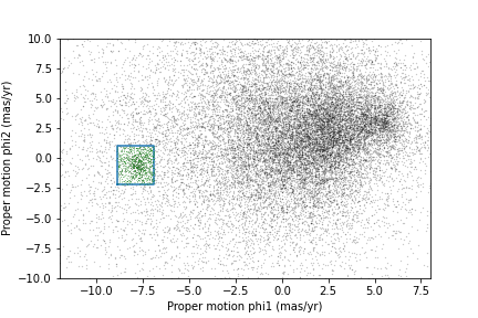

Now we will make the same plot using proper motions in the ICRS frame, which are stored in columns named pmra and pmdec.

PYTHON

x = centerline_df['pmra']
y = centerline_df['pmdec']
plt.plot(x, y, 'ko', markersize=0.3, alpha=0.3)

x = selected_df['pmra']
y = selected_df['pmdec']
plt.plot(x, y, 'gx', markersize=1, alpha=0.3)
    
plt.xlabel('Proper motion ra (ICRS frame)')
plt.ylabel('Proper motion dec (ICRS frame)')

plt.xlim([-10, 5])
plt.ylim([-20, 5]);

OUTPUT

<Figure size 432x288 with 1 Axes>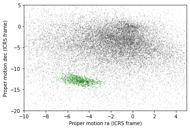

The proper motions of the selected stars are more spread out in this frame, which is why it was preferable to do the selection in the GD-1 frame.

In the following exercise, we will identify a rectangle that encompasses the majority of the stars we identified as having proper motion consistent with that of GD-1 without including too many other stars.

Exercise (5 minutes)

Looking at the proper motion of the stars we identified along the centerline of GD-1, in the ICRS reference frame define a rectangle (pmra_min, pmra_max, pmdec_min, and pmdec_max) that encompass the proper motion of the majority of the stars near the centerline of GD-1 without including to much contamination from other stars.

Show me the solution

PYTHON

pmra_min = -6.70
pmra_max = -3
pmdec_min = -14.31
pmdec_max = -11.2

Assembling the query

---

In episode 2 we used the following query to select stars in a polygonal region around a small part of GD-1 with a few filters on color and distance (parallax):

PYTHON

candidate_coord_query_base = """SELECT
{columns}
FROM gaiadr2.gaia_source
WHERE parallax < 1
  AND bp_rp BETWEEN -0.75 AND 2 
  AND 1 = CONTAINS(POINT(ra, dec), 
                   POLYGON({sky_point_list}))
"""

In this episode we will make two changes:

1. We will select stars with coordinates in a larger region to include more of GD-1.

2. We will add another clause to select stars whose proper motion is in the range we just defined in the previous exercise.

The fact that we remove most contaminating stars with the proper motion filter is what allows us to expand our query to include most of GD-1 without returning too many results. As we did in episode 2, we will define the physical region we want to select in the GD-1 frame and transform it to the ICRS frame to query the Gaia catalog which is in the ICRS frame.

Here are the coordinates of the larger rectangle in the GD-1 frame.

PYTHON

phi1_min = -70 * u.degree
phi1_max = -20 * u.degree
phi2_min = -5 * u.degree
phi2_max = 5 * u.degree

We selected these bounds by trial and error, defining the largest region we can process in a single query.

PYTHON

phi1_rect, phi2_rect = make_rectangle(
    phi1_min, phi1_max, phi2_min, phi2_max)

Here is how we transform it to ICRS, as we saw in episode 2.

PYTHON

corners = SkyCoord(phi1=phi1_rect, 
                   phi2=phi2_rect, 
                   frame=gd1_frame)

corners_icrs = corners.transform_to('icrs')

To use corners_icrs as part of an ADQL query, we have to convert it to a string. Fortunately, we wrote a function, skycoord_to_string to do this in episode 2 which we will call now.

PYTHON

sky_point_list = skycoord_to_string(corners_icrs)
sky_point_list

OUTPUT

'135.306, 8.39862, 126.51, 13.4449, 163.017, 54.2424, 172.933, 46.4726, 135.306, 8.39862'

Here are the columns we want to select.

PYTHON

columns = 'source_id, ra, dec, pmra, pmdec'

Now we have everything we need to assemble the query, but DO NOT try to run this query. Because it selects a larger region, there are too many stars to handle in a single query. Until we select by proper motion, that is.

PYTHON

candidate_coord_query = candidate_coord_query_base.format(columns=columns, 
                            sky_point_list=sky_point_list)
print(candidate_coord_query)

OUTPUT

SELECT
source_id, ra, dec, pmra, pmdec
FROM gaiadr2.gaia_source
WHERE parallax < 1
  AND bp_rp BETWEEN -0.75 AND 2 
  AND 1 = CONTAINS(POINT(ra, dec), 
                   POLYGON(135.306, 8.39862, 126.51, 13.4449, 163.017, 54.2424, 172.933, 46.4726, 135.306, 8.39862))

Selecting proper motion

---

Now we are ready to add a WHERE clause to select stars whose proper motion falls range we defined in the last exercise.

Exercise (10 minutes)

Define candidate_coord_pm_query_base, starting with candidate_coord_query_base and adding two new BETWEEN clauses to select stars whose coordinates of proper motion, pmra and pmdec, fall within the region defined by pmra_min, pmra_max, pmdec_min, and pmdec_max. In the next exercise we will use the format statement to fill in the values we defined above.

Show me the solution

PYTHON

candidate_coord_pm_query_base = """SELECT 
{columns}
FROM gaiadr2.gaia_source
WHERE parallax < 1
  AND bp_rp BETWEEN -0.75 AND 2 
  AND 1 = CONTAINS(POINT(ra, dec), 
                   POLYGON({sky_point_list}))
  AND pmra BETWEEN {pmra_min} AND  {pmra_max}
  AND pmdec BETWEEN {pmdec_min} AND {pmdec_max}
"""

Exercise (5 minutes)

Use format to format candidate_coord_pm_query_base and define candidate_coord_pm_query, filling in the values of columns, sky_point_list, and pmra_min, pmra_max, pmdec_min, pmdec_max.

Show me the solution

PYTHON

candidate_coord_pm_query = candidate_coord_pm_query_base.format(columns=columns, 
                            sky_point_list=sky_point_list,
                            pmra_min=pmra_min,
                            pmra_max=pmra_max,
                            pmdec_min=pmdec_min,
                            pmdec_max=pmdec_max)
print(candidate_coord_pm_query)

Now we can run the query like this:

PYTHON

candidate_coord_pm_job = Gaia.launch_job_async(candidate_coord_pm_query)
print(candidate_coord_pm_job)

OUTPUT

INFO: Query finished. [astroquery.utils.tap.core]
<Table length=8409>
   name    dtype    unit                              description                            
--------- ------- -------- ------------------------------------------------------------------
source_id   int64          Unique source identifier (unique within a particular Data Release)
       ra float64      deg                                                    Right ascension
      dec float64      deg                                                        Declination
     pmra float64 mas / yr                         Proper motion in right ascension direction
    pmdec float64 mas / yr                             Proper motion in declination direction
Jobid: 1616771462206O
Phase: COMPLETED
[Output truncated]

And get the results.

PYTHON

candidate_gaia_table = candidate_coord_pm_job.get_results()
len(candidate_gaia_table)

OUTPUT

8409

BETWEEN vs POLYGON

You may be wondering why we used BETWEEN for proper motion when we previously used POLYGON for coordinates. ADQL intends the POLYGON function to only be used on coordinates and not on proper motion. To enforce this, it will produce an error when a negative value is passed into the first argument.

We call the results candidate_gaia_table because it contains information from the Gaia table for stars that are good candidates for GD-1.

sky_point_list, pmra_min, pmra_max, pmdec_min, and pmdec_max are a set of selection criteria that we derived from data downloaded from the Gaia Database. To make sure we can repeat our analysis at a later date we should save this information to a file.

There are several ways we could do that, but since we are already storing data in an HDF5 file, we will do the same with these variables.

To save them to an HDF5 file we first need to put them in a Pandas object. We have seen how to create a Series from a column in a DataFrame. Now we will build a Series from scratch. We do not need the full DataFrame format with multiple rows and columns because we are only storing one string (sky_point_list). We can store each string as a row in the Series and save it. One aspect that is nice about Series is that we can label each row. To do this we need an object that can define both the name of each row and the data to go in that row. We can use a Python Dictionary for this, defining the row names with the dictionary keys and the row data with the dictionary values.

PYTHON

d = dict(sky_point_list=sky_point_list, pmra_min=pmra_min, pmra_max=pmra_max, pmdec_min=pmdec_min, pmdec_max=pmdec_max)
d

OUTPUT

{'sky_point_list': '135.306, 8.39862, 126.51, 13.4449, 163.017, 54.2424, 172.933, 46.4726, 135.306, 8.39862',
 'pmra_min': -6.7,
 'pmra_max': -3,
 'pmdec_min': -14.31,
 'pmdec_max': -11.2}

And use this Dictionary to initialize a Series.

PYTHON

point_series = pd.Series(d)
point_series

OUTPUT

sky_point_list    135.306, 8.39862, 126.51, 13.4449, 163.017, 54...
pmra_min                                                       -6.7
pmra_max                                                         -3
pmdec_min                                                    -14.31
pmdec_max                                                     -11.2
dtype: object

Now we can save our Series using to_hdf().

PYTHON

filename = 'gd1_data.hdf'
point_series.to_hdf(filename, 'point_series')

Performance Warning

You may see the previous command issue this or a similar performance warning:

OUTPUT

[...] PerformanceWarning:
your performance may suffer as PyTables will pickle object types that it cannot
map directly to c-types [inferred_type->mixed-integer,key->values] [items->None]
  point_series.to_hdf(filename, 'point_series')

This is because in the Series we just created, we are mixing variables of different types: sky_point_list is a string (text), whereas pmra_min etc. are floating point numbers. While combining different data types in a single Series is somewhat inefficient, the amount of data is small enough to not matter in this case, so this warning can be safely ignored.

Plotting one more time

---

Now we can examine the results:

PYTHON

x = candidate_gaia_table['ra']
y = candidate_gaia_table['dec']
plt.plot(x, y, 'ko', markersize=0.3, alpha=0.3)

plt.xlabel('ra (degree ICRS)')
plt.ylabel('dec (degree ICRS)');

OUTPUT

<Figure size 432x288 with 1 Axes>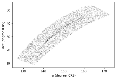

This plot shows why it was useful to transform these coordinates to the GD-1 frame. In ICRS, it is more difficult to identity the stars near the centerline of GD-1.

We can use our make_dataframe function from episode 3 to transform the results back to the GD-1 frame. In addition to doing the coordinate transformation and reflex correction for us, this function also compiles everything into a single object (a DataFrame) to make it easier to use. Note that because we put this code into a function, we can do all of this with a single line of code!

PYTHON

candidate_gaia_df = make_dataframe(candidate_gaia_table)

We can check the results using the plot_pm_selection function we wrote in episode 3.

PYTHON

plot_pm_selection(candidate_gaia_df)

OUTPUT

<Figure size 432x288 with 1 Axes>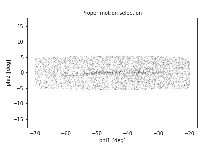

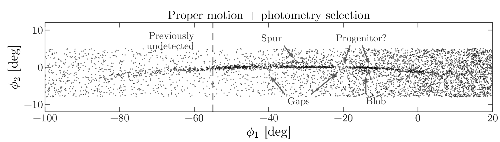
We are starting to see GD-1 more clearly. We can compare this figure with this panel from Figure 1 from the original paper:

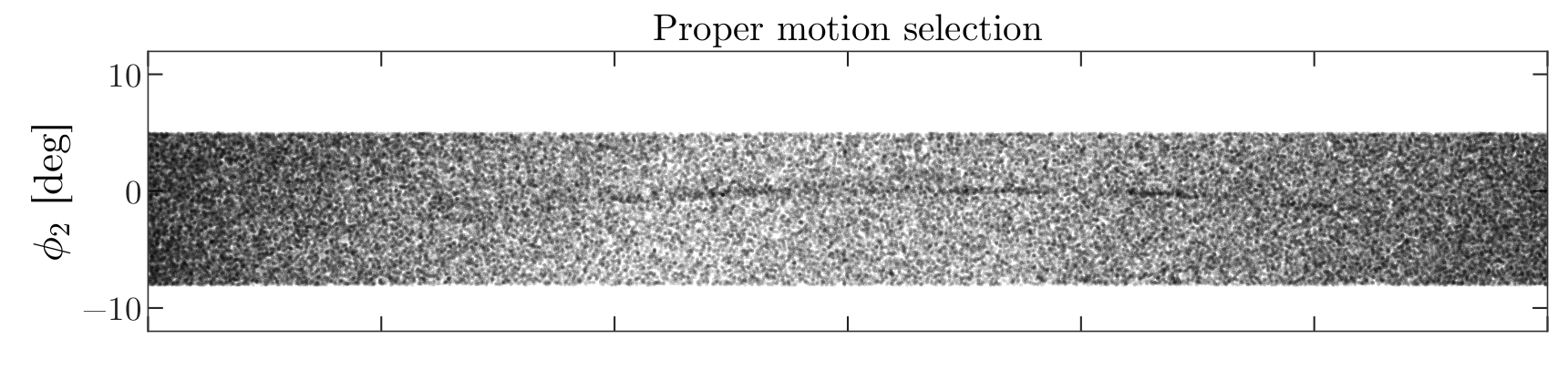
This panel shows stars selected based on proper motion only, so it is comparable to our figure (although notice that the original figure covers a wider region).

In the next episode, we will use photometry data from Pan-STARRS to do a second round of filtering, and see if we can replicate this panel.

Later we will learn how to add annotations like the ones in the figure and customize the style of the figure to present the results clearly and compellingly.

Summary

---

In the previous episode we downloaded data for a large number of stars and then selected a small fraction of them based on proper motion.

In this episode, we improved this process by writing a more complex query that uses the database to select stars based on proper motion. This process requires more computation on the Gaia server, but then we are able to either:

1. Search the same region and download less data, or

2. Search a larger region while still downloading a manageable amount of data.

In the next episode, we will learn about the database JOIN operation, which we will use in later episodes to join our Gaia data with photometry data from Pan-STARRS.

Key Points

• When possible, ‘move the computation to the data’; that is, do as much of the work as possible on the database server before downloading the data.