All Images
Basic Queries
Figure 1
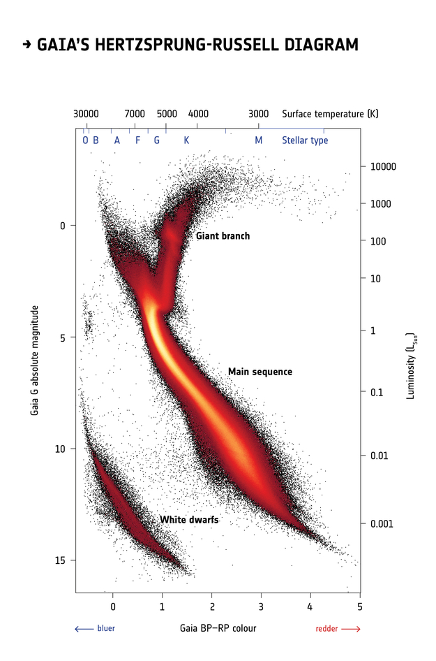
Image 1 of 1: ‘Hertzsprung-Russell diagram of BP-RP color versus luminosity.’
Coordinate Transformations
Figure 1
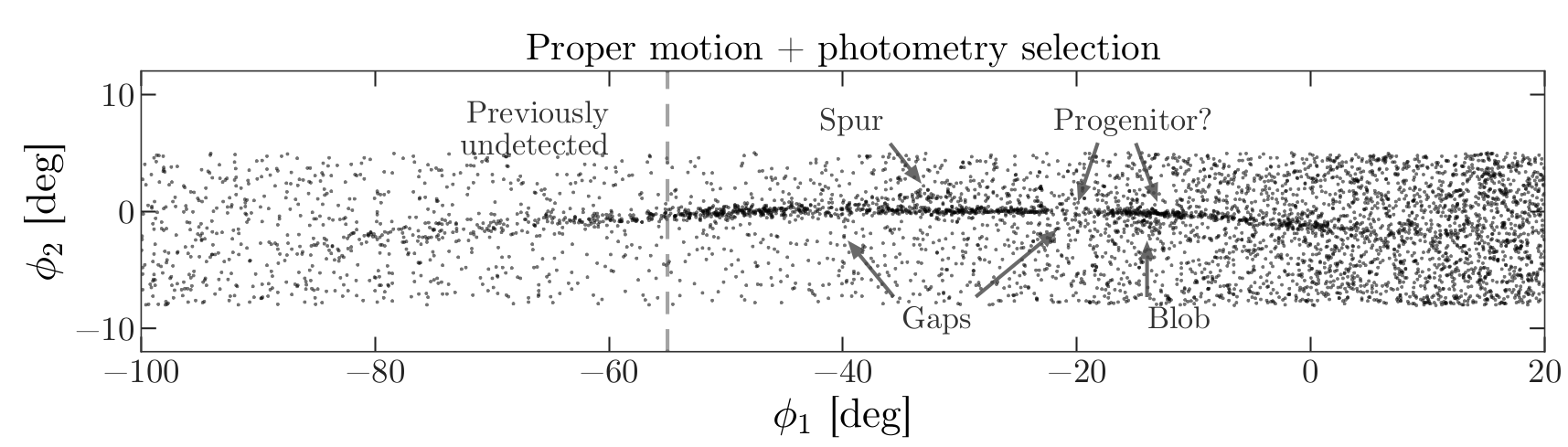
Image 1 of 1: ‘On-sky positions of likely GD-1 members in the GD-1 coordinate system, where selection by proper motion and photometry reveals the stream in great detail.’
Plotting and Tabular Data
Figure 1
Image 1 of 1: ‘Scatter plot of right ascension and declination in ICRS coordinates, demonstrating overplotting.’
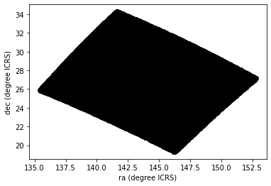
Figure 2
Image 1 of 1: ‘Scatter plot of phi1 versus phi2 in GD-1 coordinates, showing selected region is rectangular.’
Plotting and pandas
Figure 1
Image 1 of 1: ‘Scatter of proper motion phi1 versus phi2 showing overdensity in negative proper motions of GD-1 stars.’
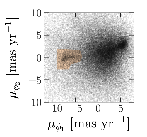
Figure 2
Image 1 of 1: ‘Scatter plot of proper motion in GD-1 frame of selected stars showing most are near the origin.’
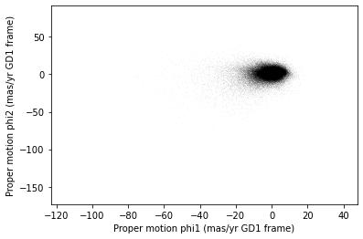
Figure 3
Image 1 of 1: ‘Zoomed in view of previous scatter plot showing overdense region.’
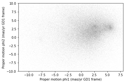
Figure 4
Image 1 of 1: ‘Scatter plot with selection on proper motion and photometry showing many stars in GD-1 are within 1 degree of phi2 = 0.’
Figure 5
Image 1 of 1: ‘Scatter plot of proper motion of selected stars showing cluster near (-7.5, 0).’
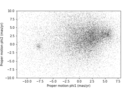
Figure 6
Image 1 of 1: ‘Scatter plot of proper motion with overlaid polygon showing overdense region selected for analysis in Price-Whelan and Bonaca paper.’
Figure 7
Image 1 of 1: ‘Scatter plot of proper motion with blue box showing overdense region selected for our analysis.’
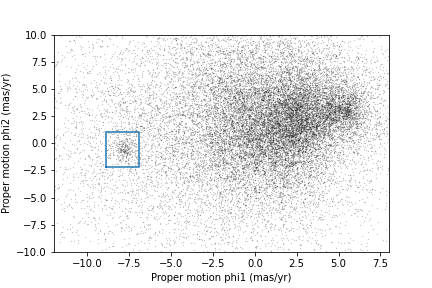
Figure 8
Image 1 of 1: ‘Scatter plot of coordinates of stars in selected region, showing tidal stream.’
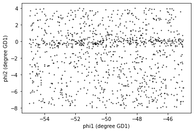
Figure 9
Image 1 of 1: ‘Scatter plot of coordinates of stars in selected region, showing tidal stream with equally proportioned axes.’
Transform and Select
Figure 1
Image 1 of 1: ‘Proper motion of stars in GD-1, showing selected region as blue box and stars within selection as green points.’
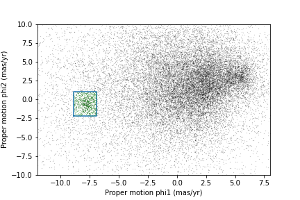
Figure 2
Image 1 of 1: ‘Proper motion in ICRS frame, showing selected stars are more spread out in this frame.’
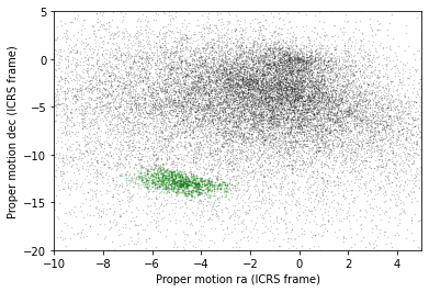
Figure 3
Image 1 of 1: ‘Scatter plot of right ascension and declination of selected stars in ICRS frame.’
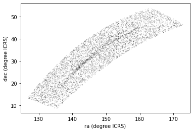
Figure 4
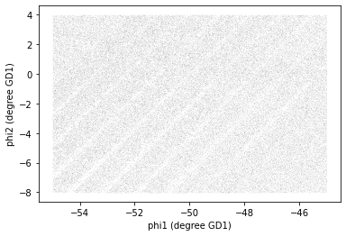
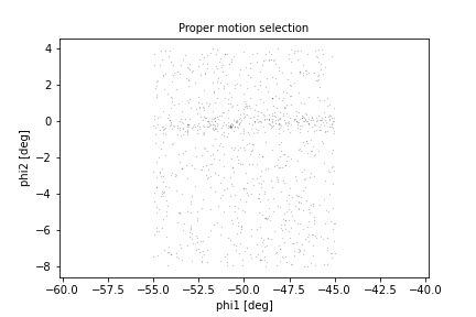
Image 1 of 1: ‘Scatter plot of phi1 versus phi2 in GD-1 frame after selecting on proper motion.’
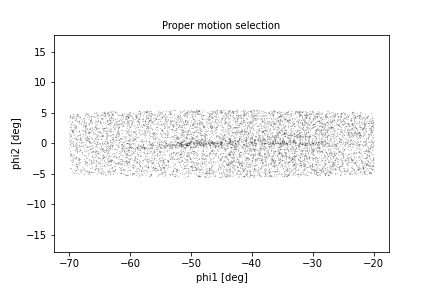
Figure 5
Image 1 of 1: ‘Figure from Price-Whelan and Bonaca paper showing phi1 vs phi2 in GD-1 after selecting on proper motion.’
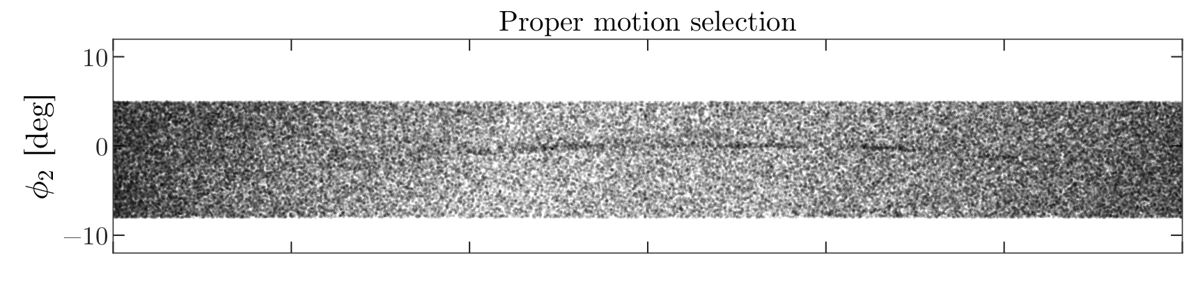
Figure 6
Image 1 of 1: ‘Figure from Price-Whelan and Bonaca paper showing phi1 vs phi2 in GD-1 after selecting on proper motion and photometry.’
Join
Figure 1
Image 1 of 1: ‘Color-magnitude diagram for the stars selected based on proper motion, from Price-Whelan and Bonaca paper.’
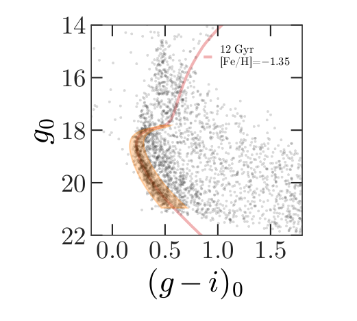
Figure 2
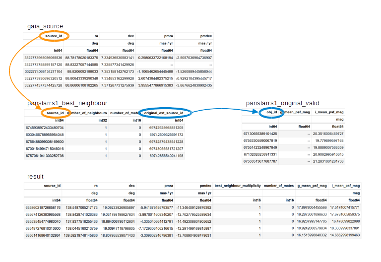
Image 1 of 1: ‘Diagram showing relationship between the gaia_source, panstarrs1_best_neighbour, and panstarrs1_original_valid tables and result table.’
Photometry
Figure 1
Image 1 of 1: ‘Color-magnitude diagram for the stars selected based on proper motion, from Price-Whelan and Bonaca paper.’
Figure 2
Image 1 of 1: ‘Color-magnitude diagram for the stars selected based on proper motion, from Price-Whelan and Bonaca paper.’
Figure 3
Image 1 of 1: ‘Color magnitude diagram of our selected stars showing all of the stars selected’
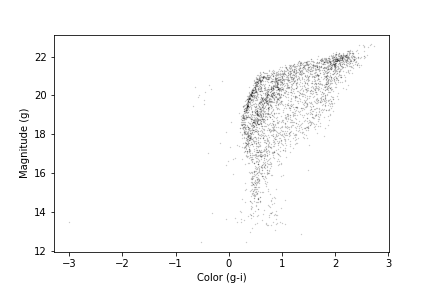
Figure 4
Image 1 of 1: ‘Color magnitude diagram of our selected stars showing overdense region in lower left.’
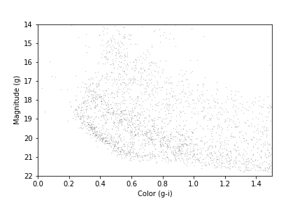
Figure 5
Image 1 of 1: ‘Color magnitude diagram of our selected stars showing overdense region in lower left.’
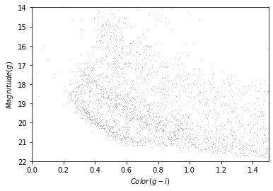
Figure 6
Image 1 of 1: ‘Color magnitude diagram of our selected stars with theoretical isochrone overlaid as blue curve.’
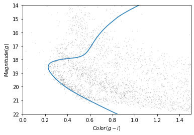
Figure 7
Image 1 of 1: ‘Color magnitude diagram of our selected stars showing left boundary as blue curve and right boundary as orange curve.’
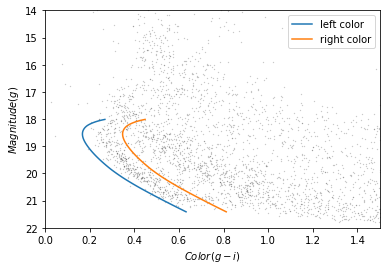
Figure 8
Image 1 of 1: ‘Color magnitude diagram of our selected stars showing polygon defined by boundaries as blue curve.’
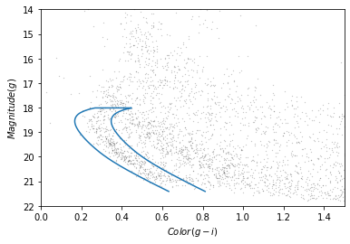
Figure 9
Image 1 of 1: ‘Color magnitude diagram showing our selected stars in green, inside our polygon.’
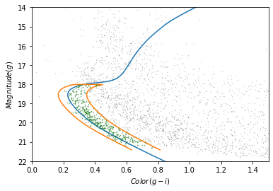
Figure 10
Image 1 of 1: ‘phi 1 and phi 2 of selected stars in the GD-1 frame after selecting for both proper motion and photometry.’
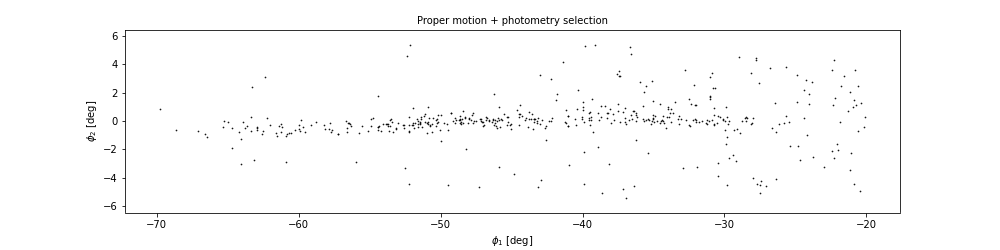
Figure 11
Image 1 of 1: ‘phi 1 and phi 2 of selected stars in the GD-1 frame after selecting for both proper motion and photometry.’
Visualization
Figure 1
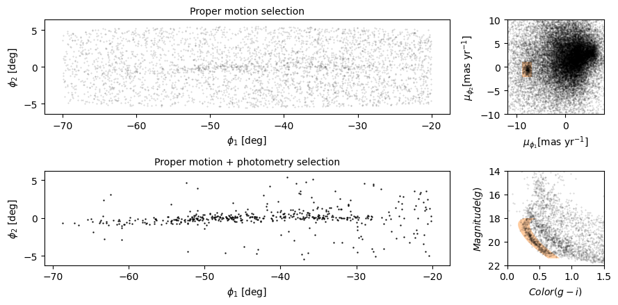
Image 1 of 1: ‘Figure 1 from Price-Whelan and Bonaca paper with four panels and caption. Caption reads: On-sky positions of likely GD-1 members in the GD-1 coordinate system. GD-1 is apparent as an overdensity in negative proper motions (top-right panel, orange box), so selecting on proper motion already reveals the stream in positions of individual stars (top-left panel). The stream also stands out in the color–magnitude diagram (bottom-right panel) as older and more metal-poor than the background. Selecting the main sequence of GD-1 (orange, shaded region in the bottom-right panel) along with proper motion cuts unveils the stream in unprecedented detail (bottom-left panel).’
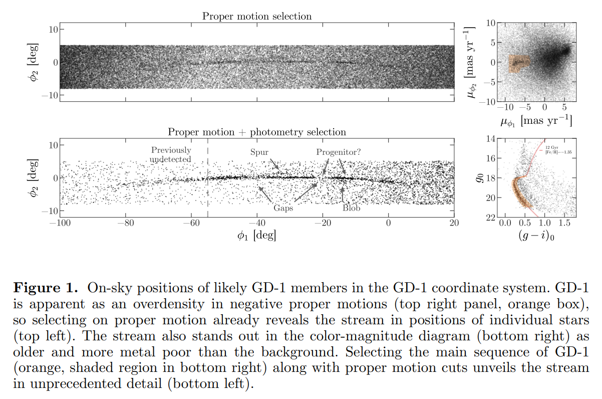
Figure 2
Image 1 of 1: ‘Four paneled plot showing our first recreation of figure 1 from the Price-Whelan and Bonaca paper.’
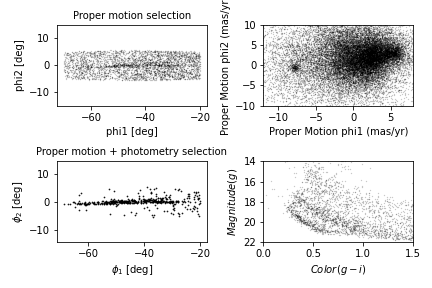
Figure 3
Image 1 of 1: ‘Four paneled plot we created above with two left-hand panels increased in width.’
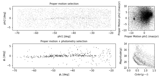
Figure 4
Image 1 of 1: ‘An orange rectangle at the coordinates used to select stars based on proper motion.’
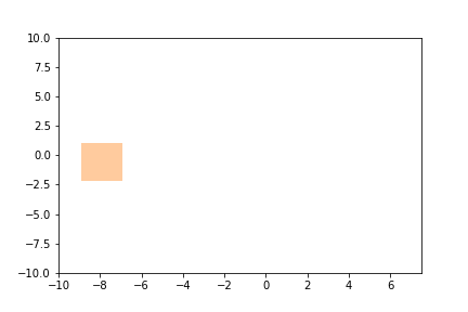
Figure 5
Image 1 of 1: ‘Proper motion with overlaid polygon showing our selected stars.’
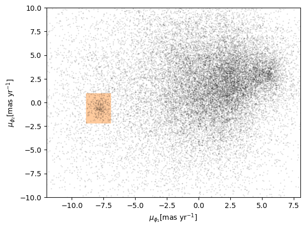
Figure 6
Image 1 of 1: ‘Four paneled plot we created above with two left-hand panels increased in width.’